Introduction to Deep Learning with Keras and tensorFlow
Introduction
Keras is an open-source software library that provides a Python interface for artificial neural networks. It works with TensorFlow, JAX, and PyTorch interchangeably.
Keras, as a high level library, allows to easily define complex ANN architectures to experiment on your data. Keras also supports GPU, which becomes essential for processing huge amount of data and developing machine learning models.
Among Keras characteristics that make it an attractive option for DL are: - User friendly, with a simple, consistent interface optimized for common use cases - Modular and Composable, with easy to connect configutrable building-blocks - Easy to extend, adding new moduels and classes
Installation and Setup
Keras runs on top of TensorFlow, which can be installed using pip:
pip install tensorflow
Once TensorFlow is installed, Keras can be accessed directly as tensorflow.keras.
Keras with Multiple Backends: JAX, TensorFlow, and PyTorch
Starting with Keras 3, the Keras API supports running the same code with different computation engines called backends. You can choose between:
"tensorflow" → uses TensorFlow as the backend.
"jax" → uses JAX, a high-performance numerical computing library from Google.
"torch" → uses PyTorch as the backend.
What is a backend?
The backend is the engine that performs the mathematical operations and model training. In earlier versions, Keras relied only on TensorFlow (via tensorflow.keras). Now, you can switch backends without changing your model code.
What does “backend-agnostic” mean?
It means that the code you write using keras.Model, keras.layers.Dense, etc., works the same regardless of the backend. You can swap the backend and the entire notebook will still run without changes.
How to set the backend
You can set the backend in your script using:
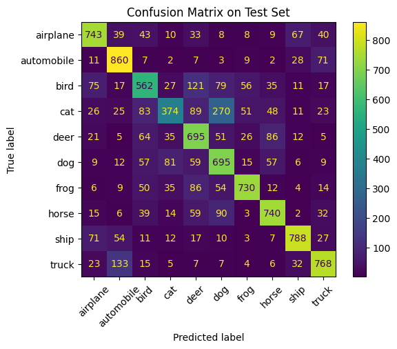
import keraskeras.config.set_backend("tensorflow") # or "jax" or "torch"## The problem to solveIn this lab we build a simple Convolutional Neural Network to classify images using theCIFAR-10 dataset.The CIFAR-10 dataset is a collection of images commonly used for training machine learning and computer vision models.It consists of 60000 color images divided into 10 different classes. Each image is32 by 32 pixels in size and has three color channels red, green, and blue.The dataset is split into 50000 training images and10000 test images.The 10 classes represent different object categories:airplane, automobile, bird, cat, deer, dog, frog, horse, ship, and truck.CIFAR-10is widely used as a benchmark for image classification tasks due to its manageable size and variety of image content.## Keras Workflow OverviewKeras follows a simple and consistent workflow that makes it easy to build and train deep learning models. Below are the typical steps you will follow when working with Keras:1.**Importing libraries and loading data** Load and preprocess the dataset, including normalization and label encoding if needed.2.**Defining the model** Choose the model architecture using either the Sequential or Functional API, and add layers.3.**Compiling the model** Specify the loss function, optimizer, and evaluation metrics.4.**Training the model** Use the `fit()` method to train the model with training data. You can also include validation data, callbacks, and early stopping.5.**Evaluating the model** Use the `evaluate()` method to measure performance on a test set.6.**Making predictions** Use the `predict()` method on new or unseen data.7.**Saving and loading the model** Save your trained model to reuse later or deploy it in production.8.**(Optional) Tuning and visualization** Monitor training progress with plots or tools like TensorBoard, and tune hyperparameters for better performance.## Step 1a: Import Libraries::: {#5de7e855 .cell}``` {.python .cell-code}import tensorflow as tffrom tensorflow.keras import layers, modelsfrom tensorflow.keras.datasets import cifar10from tensorflow.keras.utils import to_categoricalfrom sklearn.metrics import confusion_matrix, ConfusionMatrixDisplayimport matplotlib.pyplot as pltimport numpy as npimport osimport datetime
:::
## Step 1b: Load Data
# Load CIFAR-10 dataset(x_train, y_train), (x_test, y_test) = cifar10.load_data()# Normalize pixel values to the range [0, 1]x_train, x_test = x_train /255.0, x_test /255.0# Convert class labels to one-hot encodingy_train_cat = to_categorical(y_train, 10)y_test_cat = to_categorical(y_test, 10)
---------------------------------------------------------------------------NameError Traceback (most recent call last)
Cell In[1], line 2 1# Load CIFAR-10 dataset----> 2 (x_train, y_train), (x_test, y_test) =cifar10.load_data()
4# Normalize pixel values to the range [0, 1] 5 x_train, x_test = x_train /255.0, x_test /255.0NameError: name 'cifar10' is not defined
Step 2: Define the Model
We define a simple convolutional neural network using the Keras Sequential API. The model includes convolutional and pooling layers, followed by dense layers.
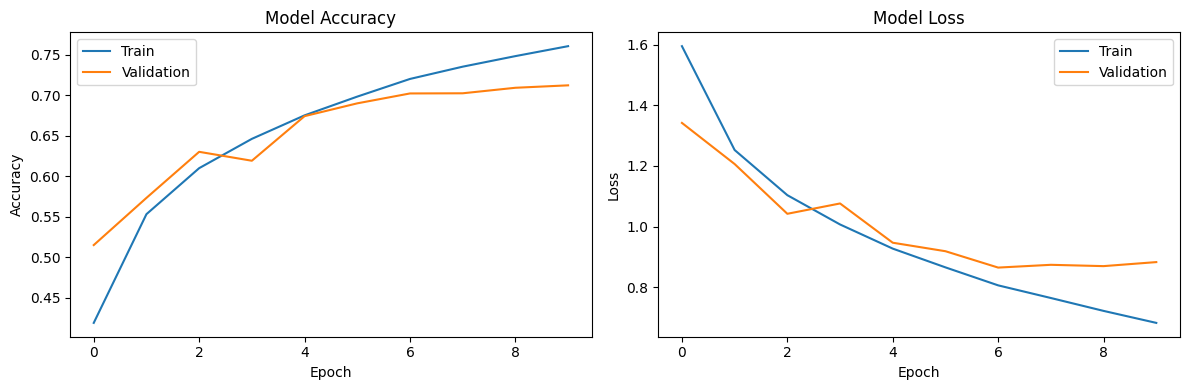
We train the model using the fit method with a validation split, and apply the callbacks we defined earlier.
history = model.fit( x_train, y_train_cat, epochs=20, batch_size=64, validation_split=0.1, callbacks=[tensorboard_callback, early_stop, checkpoint], verbose=2)# Save the trained model for further usemodel.save("cnn_cifar10_model.keras")