The caret package

Authors

Esteban Vegas

Ferran Reverter

Alex Sanchez

Published

March 24, 2025

options(width=100) 
if(!require("knitr")) install.packages("knitr")
library("knitr")
#getOption("width")
knitr::opts_chunk$set(comment=NA,echo = TRUE, cache=TRUE)

Introduction to `caret`

if(!require("caret")) install.packages("caret")
if(!require("mlbench")) install.packages("mlbench")
library("caret")

The caret package, short for classification and regression training, was built with several goals in mind:

Create a unified interface for modelling and prediction (interfaces to more than 200 models),
Develop a set of semi-automated, reasonable approaches for optimizing the values of the tuning parameters for many of these models and
Increase computational efficiency using parallel processing.

That is caret has been developed to facilitate building, evaluating and comparing predictive models and as such it is an interesting alternative to using multiple different packages for distinct tasks, which, not only requires more time to learn how to use each of them, but especially makes it much harder to compare them.

Learning to use `caret`

There are multiple resources to learn caretthat go from simple tutorials like this one or similars to courses, papers and a book by Max Kuhn, the creator or the package.

Guiding example

The caret package can be used to perform a study from beginning to end.
For this, it implements a set of general functions that can roughly be associated with the distinct steps of an analytical pipeline.
We follow an example based on the sonar data from the mlbench package to illustrate the multiple functionalities of the package .

The goal is to predict two classes:

M for metal cylinder
R for rock

Data loading

library("mlbench")
data(Sonar)
names(Sonar)

 [1] "V1"    "V2"    "V3"    "V4"    "V5"    "V6"    "V7"    "V8"    "V9"    "V10"   "V11"   "V12"  
[13] "V13"   "V14"   "V15"   "V16"   "V17"   "V18"   "V19"   "V20"   "V21"   "V22"   "V23"   "V24"  
[25] "V25"   "V26"   "V27"   "V28"   "V29"   "V30"   "V31"   "V32"   "V33"   "V34"   "V35"   "V36"  
[37] "V37"   "V38"   "V39"   "V40"   "V41"   "V42"   "V43"   "V44"   "V45"   "V46"   "V47"   "V48"  
[49] "V49"   "V50"   "V51"   "V52"   "V53"   "V54"   "V55"   "V56"   "V57"   "V58"   "V59"   "V60"  
[61] "Class"

The sonarpackage has 208 data points collected on 60 predictors (energy within a particular frequency band).

Train/test splitting

We will most of the time want to split the data into two groups: a training set and a test set.

This may be done with the createDataPartition function:

set.seed(1234) # Control of data generation
inTrain <- createDataPartition(y=Sonar$Class, p=.75, list=FALSE)
str(inTrain)

 int [1:157, 1] 2 3 4 6 7 8 9 11 14 15 ...
 - attr(*, "dimnames")=List of 2
  ..$ : NULL
  ..$ : chr "Resample1"

training <- Sonar[inTrain,]
testing <- Sonar[-inTrain,]
nrow(training)

[1] 157

Others similar functions are: createFolds and createResample,

Preprocessing and training

Usually, before prediction, data may have to be cleaned and pre-processed.

Caret allows to integrate it with the training step using the train function.

This function has multiple parameter such as:

method: Can choose from more than 200 models
preprocess: all type of filtering and transformations

CART1Model <- train (Class ~ ., 
                   data=training, 
                   method="rpart1SE",
                   preProc=c("center","scale"))
CART1Model

CART 

157 samples
 60 predictor
  2 classes: 'M', 'R' 

Pre-processing: centered (60), scaled (60) 
Resampling: Bootstrapped (25 reps) 
Summary of sample sizes: 157, 157, 157, 157, 157, 157, ... 
Resampling results:

  Accuracy   Kappa   
  0.6752493  0.350363

Refining specifications

Many specifications can be passed using the trainControl instruction.

ctrl <- trainControl(method = "repeatedcv", repeats=3)
CART1Model3x10cv <- train (Class ~ ., 
                         data=training, 
                         method="rpart1SE",
                         trControl=ctrl,
                         preProc=c("center","scale"))

CART1Model3x10cv

CART 

157 samples
 60 predictor
  2 classes: 'M', 'R' 

Pre-processing: centered (60), scaled (60) 
Resampling: Cross-Validated (10 fold, repeated 3 times) 
Summary of sample sizes: 141, 142, 142, 141, 141, 142, ... 
Resampling results:

  Accuracy   Kappa    
  0.7087173  0.4168066

We can change the method used by changing the trainControl parameter.

In the example below we fit a classification tree with different options:

ctrl <- trainControl(method = "repeatedcv", repeats=3,
                     classProbs=TRUE,
                     summaryFunction=twoClassSummary)

CART1Model3x10cv <- train (Class ~ ., 
                         data=training, 
                         method="rpart1SE", 
                         trControl=ctrl, 
                         metric="ROC", 
                         preProc=c("center","scale"))

CART1Model3x10cv

CART 

157 samples
 60 predictor
  2 classes: 'M', 'R' 

Pre-processing: centered (60), scaled (60) 
Resampling: Cross-Validated (10 fold, repeated 3 times) 
Summary of sample sizes: 141, 141, 142, 141, 141, 142, ... 
Resampling results:

  ROC        Sens   Spec     
  0.7757068  0.775  0.6869048

CART2Fit3x10cv <- train (Class ~ ., 
                       data=training, 
                       method="rpart", 
                       trControl=ctrl, 
                       metric="ROC", 
                       preProc=c("center","scale"))
CART2Fit3x10cv

CART 

157 samples
 60 predictor
  2 classes: 'M', 'R' 

Pre-processing: centered (60), scaled (60) 
Resampling: Cross-Validated (10 fold, repeated 3 times) 
Summary of sample sizes: 142, 142, 142, 142, 142, 140, ... 
Resampling results across tuning parameters:

  cp          ROC        Sens       Spec     
  0.06849315  0.7033441  0.6851852  0.6779762
  0.10958904  0.6829282  0.7523148  0.5922619
  0.47945205  0.5517196  0.8629630  0.2404762

ROC was used to select the optimal model using the largest value.
The final value used for the model was cp = 0.06849315.

plot(CART2Fit3x10cv)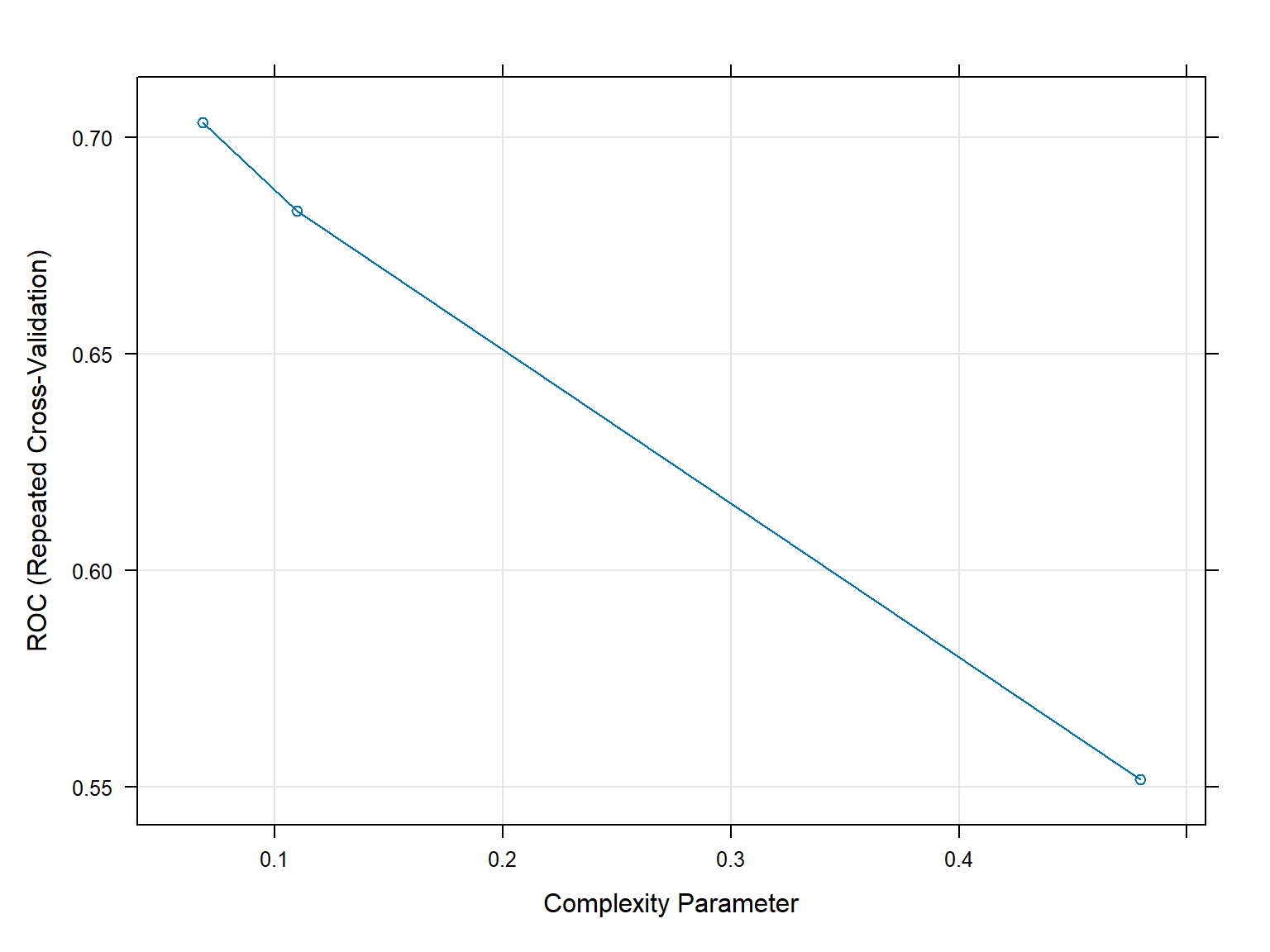

CART2Fit3x10cv <- train (Class ~ ., 
                       data=training, 
                       method="rpart", 
                       trControl=ctrl, 
                       metric="ROC",  
                       tuneLength=10,
                       preProc=c("center","scale"))
CART2Fit3x10cv

CART 

157 samples
 60 predictor
  2 classes: 'M', 'R' 

Pre-processing: centered (60), scaled (60) 
Resampling: Cross-Validated (10 fold, repeated 3 times) 
Summary of sample sizes: 141, 142, 140, 141, 141, 142, ... 
Resampling results across tuning parameters:

  cp          ROC        Sens       Spec     
  0.00000000  0.7375744  0.7305556  0.6220238
  0.05327245  0.7382523  0.7453704  0.6130952
  0.10654490  0.6816468  0.7773148  0.5696429
  0.15981735  0.6787368  0.8092593  0.5482143
  0.21308980  0.6787368  0.8092593  0.5482143
  0.26636225  0.6787368  0.8092593  0.5482143
  0.31963470  0.6787368  0.8092593  0.5482143
  0.37290715  0.6787368  0.8092593  0.5482143
  0.42617960  0.6787368  0.8092593  0.5482143
  0.47945205  0.5748016  0.8680556  0.2815476

ROC was used to select the optimal model using the largest value.
The final value used for the model was cp = 0.05327245.

plot(CART2Fit3x10cv)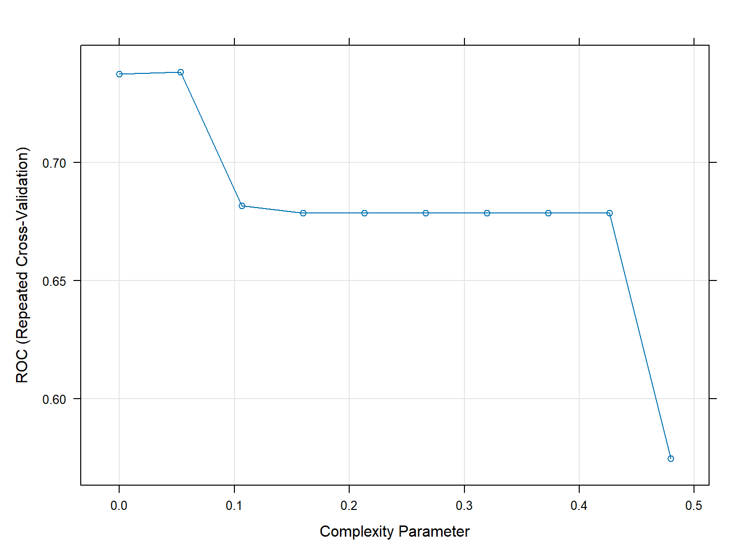

Predict & confusionMatrix functions

To predict new samples can be used predict function.

type = prob : to compute class probabilities
type = raw : to predict the class

The confusionMatrix function will compute the confusion matrix and associated statistics for the model fit.

CART2Probs <- predict(CART2Fit3x10cv, newdata = testing, type = "prob")
CART2Classes <- predict(CART2Fit3x10cv, newdata = testing, type = "raw")
confusionMatrix(data=CART2Classes,testing$Class)

Confusion Matrix and Statistics

          Reference
Prediction  M  R
         M 21  5
         R  6 19
                                          
               Accuracy : 0.7843          
                 95% CI : (0.6468, 0.8871)
    No Information Rate : 0.5294          
    P-Value [Acc > NIR] : 0.0001502       
                                          
                  Kappa : 0.5681          
                                          
 Mcnemar's Test P-Value : 1.0000000       
                                          
            Sensitivity : 0.7778          
            Specificity : 0.7917          
         Pos Pred Value : 0.8077          
         Neg Pred Value : 0.7600          
             Prevalence : 0.5294          
         Detection Rate : 0.4118          
   Detection Prevalence : 0.5098          
      Balanced Accuracy : 0.7847          
                                          
       'Positive' Class : M

Model comparison

The resamplesfunction enable smodel comparison

resamps=resamples(list(CART2=CART2Fit3x10cv,
                       CART1=CART1Model3x10cv))
summary(resamps)


Call:
summary.resamples(object = resamps)

Models: CART2, CART1 
Number of resamples: 30 

ROC 
           Min.   1st Qu.    Median      Mean   3rd Qu.     Max. NA's
CART2 0.5000000 0.6294643 0.7455357 0.7382523 0.8058036 0.952381    0
CART1 0.5535714 0.7249504 0.7926587 0.7757068 0.8315972 0.937500    0

Sens 
           Min.   1st Qu.    Median      Mean 3rd Qu. Max. NA's
CART2 0.4444444 0.6250000 0.7500000 0.7453704   0.875    1    0
CART1 0.4444444 0.6666667 0.7777778 0.7750000   0.875    1    0

Spec 
       Min.   1st Qu.    Median      Mean   3rd Qu.      Max. NA's
CART2 0.250 0.5714286 0.6250000 0.6130952 0.7142857 0.8750000    0
CART1 0.375 0.5714286 0.7142857 0.6869048 0.8571429 0.8571429    0

xyplot(resamps,what="BlandAltman")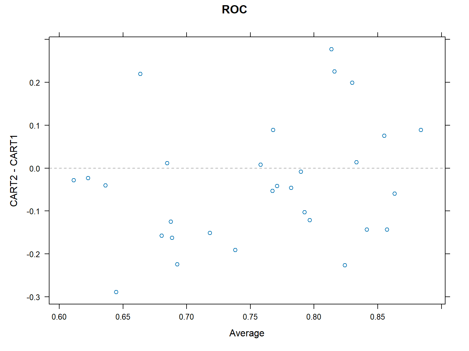

diffs<-diff(resamps)
summary(diffs)


Call:
summary.diff.resamples(object = diffs)

p-value adjustment: bonferroni 
Upper diagonal: estimates of the difference
Lower diagonal: p-value for H0: difference = 0

ROC 
      CART2  CART1   
CART2        -0.03745
CART1 0.1598         

Sens 
      CART2  CART1   
CART2        -0.02963
CART1 0.4514         

Spec 
      CART2   CART1   
CART2         -0.07381
CART1 0.02404

Example: Comparison of boosting methods

We use the caret package and the BreastCancer dataset.

Adaboost

In this example, we are using the rpart algorithm as the base learner for AdaBoost. We can then use the predict function to make predictions on new data:

library(caret)
library(mlbench)

data(BreastCancer)

# Split the data into training and testing sets
set.seed(123)
trainIndex <- createDataPartition(BreastCancer$Class, p = 0.7, list = FALSE)
training <- BreastCancer[trainIndex, ]
testing <- BreastCancer[-trainIndex, ]

# Next, set up 
# - the training control and 
# - tuning parameters for the AdaBoost algorithm:

ctrl <- trainControl(method = "repeatedcv", 
                     number = 10, repeats = 3,
                     classProbs = TRUE, 
                     summaryFunction = twoClassSummary)

params <- data.frame(method = "AdaBoost", 
                     nIter = 100, 
                     interaction.depth = 1, 
                     shrinkage = 0.1)

#  we are using 10-fold cross-validation with 3 repeats and the twoClassSummary function for evaluation. 
# We are also setting the number of iterations for the AdaBoost algorithm to 100, the maximum interaction depth to 1, and the shrinkage factor to 0.1.

# Use the train function to train the AdaBoost algorithm on the training data and evaluate its performance on the testing data:

adaboost <- train(Class ~ ., data = training, 
                  method = "rpart", 
                  trControl = ctrl, 
                  tuneGrid = params)

predictions <- predict(adaboost, newdata = testing)

# Evaluate the performance of the model
confusionMatrix(predictions, testData$diagnosis)

Gradient boosting

We use the gbm method in train() function from the caret package to build a Gradient Boosting model on the Breast Cancer dataset.

library(caret)
library(gbm)
data(BreastCancer)

# Convert the diagnosis column to a binary factor
BreastCancer$diagnosis <- ifelse(BreastCancer$diagnosis == "M", 1, 0)

# Split the dataset into training and testing sets
trainIndex <- createDataPartition(BreastCancer$diagnosis, p = 0.7, list = FALSE)
trainData <- BreastCancer[trainIndex, ]
testData <- BreastCancer[-trainIndex, ]

# Define the training control
ctrl <- trainControl(method = "cv", number = 10, classProbs = TRUE, summaryFunction = twoClassSummary)

# Define the Gradient Boosting model
model <- train(diagnosis ~ ., data = trainData, method = "gbm", trControl = ctrl,
               verbose = FALSE, metric = "ROC", n.trees = 1000, interaction.depth = 3, shrinkage = 0.01)

# Make predictions on the testing set
predictions <- predict(model, testData)

# Evaluate the performance of the model
confusionMatrix(predictions, testData$diagnosis)

XGBoost

In this example, we use the xgbTree method in train() function from the caret package to build an XGBoost model on the BreastCancer dataset.
The hyperparameters are set to default values, except for parameters:
- nrounds,
- max_depth,
- eta, lambda, and
- alpha
The final performance is evaluated using a confusion matrix.

library(caret)
library(xgboost)
data(BreastCancer)

# Convert the diagnosis column to a binary factor
BreastCancer$diagnosis <- ifelse(BreastCancer$diagnosis == "M", 1, 0)

# Split the dataset into training and testing sets
trainIndex <- createDataPartition(BreastCancer$diagnosis, p = 0.7, list = FALSE)
trainData <- BreastCancer[trainIndex, ]
testData <- BreastCancer[-trainIndex, ]

# Define the training control
ctrl <- trainControl(method = "cv", number = 10, classProbs = TRUE, summaryFunction = twoClassSummary)

# Define the XGBoost model
model <- train(diagnosis ~ ., 
               data = trainData, 
               method = "xgbTree", trControl = ctrl,
               verbose = FALSE, metric = "ROC", 
               nrounds = 1000, max_depth = 3, 
               eta = 0.01, lambda = 1, alpha = 0)

# Make predictions on the testing set
predictions <- predict(model, testData)

# Evaluate the performance of the model
confusionMatrix(predictions, testData$diagnosis)

The caret package

Introduction to `caret`

Learning to use `caret`

Guiding example

Data loading

Train/test splitting

Preprocessing and training

Refining specifications

Predict & confusionMatrix functions

Model comparison

Example: Comparison of boosting methods

Adaboost

Gradient boosting

XGBoost

References

Official references and resources

Other resources

Introduction to caret

Learning to use caret

Guiding example

Data loading

Train/test splitting

Preprocessing and training

Refining specifications

Predict & confusionMatrix functions

Model comparison

Example: Comparison of boosting methods

Adaboost

Gradient boosting

XGBoost

References

Official references and resources

Other resources

Introduction to `caret`

Learning to use `caret`