ARTIFICIAL NEURAL NETWORKS
Neural Networks, Deep Learning and
Artificial Intelligence
From Artificial Neural Networks to Artifial Intelligence
Historical Background (1)
In the post-pandemic world, a lightning rise of AI, with a mess of realities and promises is impacting society.
Since the emergence -and rapid growth- of Large Language Models and Generative AI everybody has an experience, an opinion, or a fear on the topic.
Is it just machine learning?
Many tasks performed by AI can be described as Predictive as seen in Recommendation systems, Image recognition or Natural language processing.
However, AI is broader than just prediction systems
Generative AI is also able to generate new content.
Both, predictive and generative capabilities of AI have far-reaching implications beyond technologies, including ethical or social aspects.
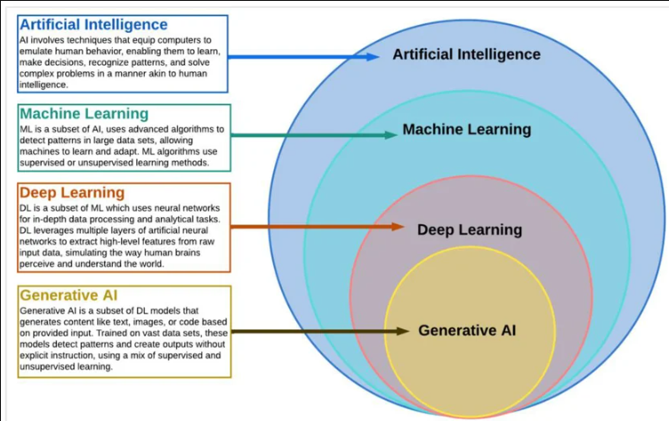
AI, ANNs and Deep learning
In many contexts, talking about AI means talking about Deep Learning (DL).
DL is the dominant paradigm in modern (2026) AI and is behind applications such as self-driving cars, voice assistants, and medical diagnosis systems.
DL originates in the field of Artificial Neural Networks
DL extends the basic principles of ANNs by:
- Adding complex architectures and algorithms and
- Enabling scalable learning from large data
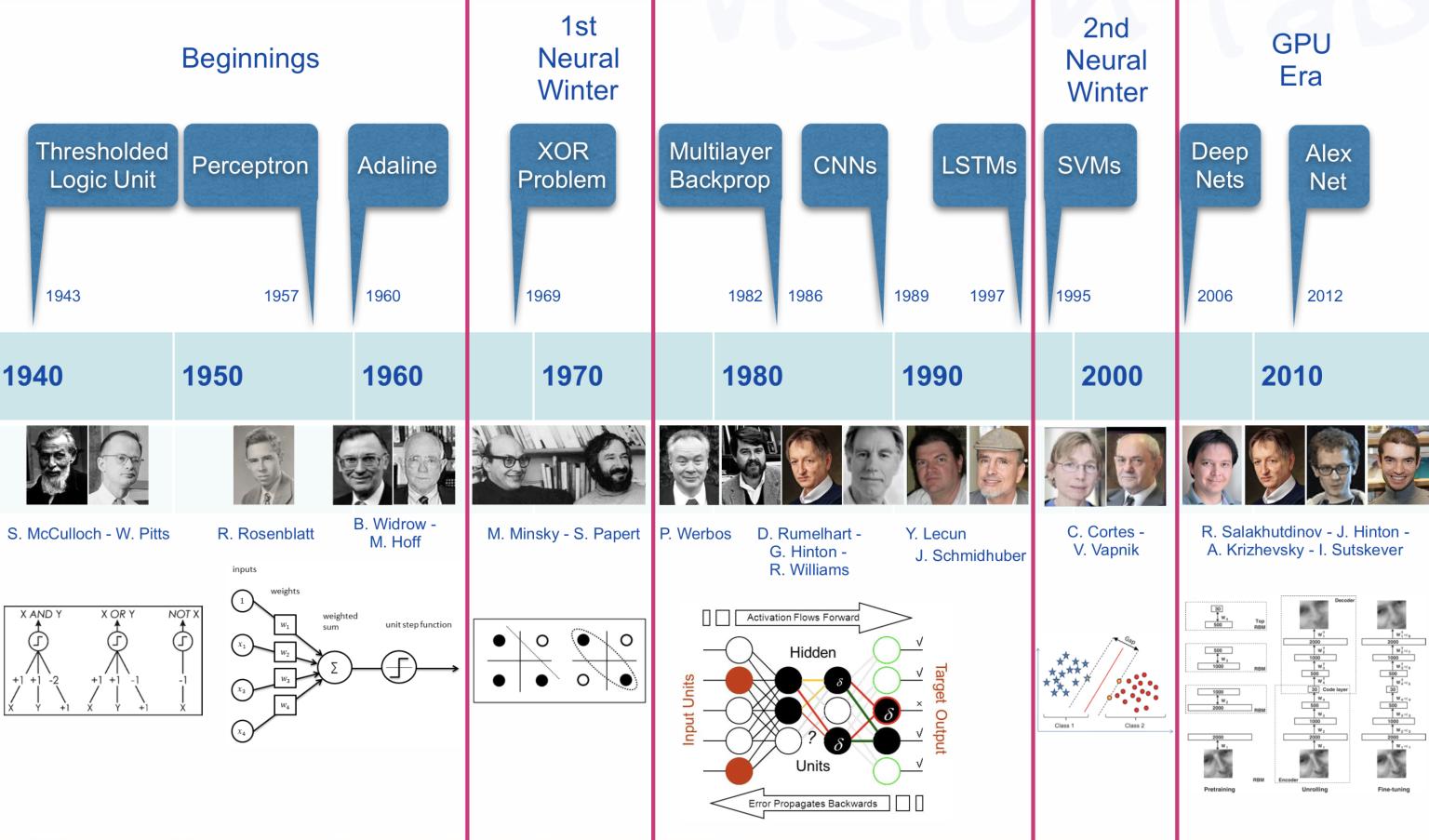
The early history of AI (1)
From ANN to Deep learning
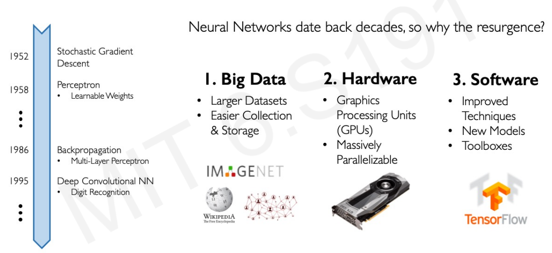
Why Deep Learning Now?
How does it all fit?
Size does matter!

Performance comparison between Deep Learning and other ML algorithms
DL modeling from large amounts of data can increase the performance
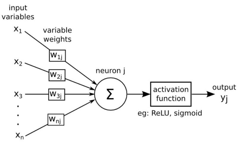
The Artificial Neurone
Emulating biological neurons

- First model of an artifial neurone proposed by Mc Cullough & Pitts in 1943
- They aimed at building a mathematical model of a neurone.
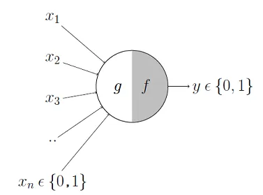
Mc Cullough’s neuron
The neuron can be divided into two parts:
- \(g\): combines the input signals,
- \(f\): yields final output from the aggregated value.
The neuron computes: \[ y = f(g(x_1,\dots,x_n)). \]
- The neuron first aggregates, \(g()\), the inputs, \(\mathbb(x)\), and then
- Applies decision rule \(f()\) to produce a binary output \(y \in \{0,1\}\).
From the AN to the perceptron
Mc Cullogh’s neuron has important limitations:
- Inputs are binary: \(x_i \in \{0,1\}\)
- All inputs are treated in a fixed way
- The decision rule is rigid (fixed threshold)
To build more flexible the perceptron was introduced.
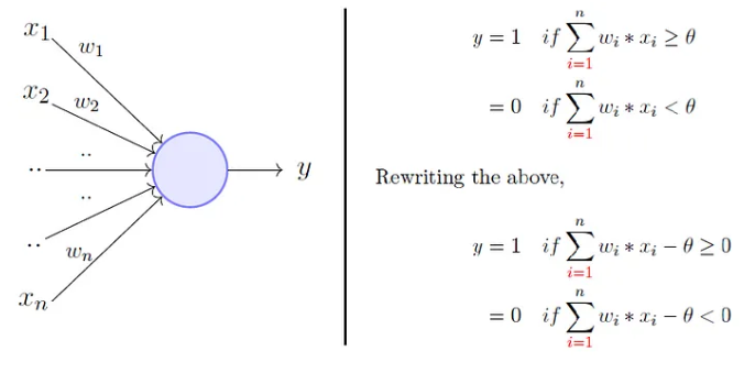
The Perceptron
To overcome Mc Cullogh’s neuron limitations Rosenblatt, proposed the perceptron model, or artificial neuron, in 1958.
It generalizes previous one in that weights and thresholds can be learnt over time.
- It takes a weighted sum of the inputs and
- It sets the output to 1 if the weighted sum exceeds a threshold \(\theta\), and to 0 otherwise.
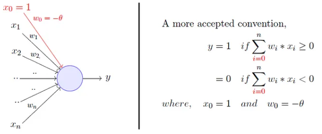
Rosenblatt’s perceptron
Rosenblatt’s perceptron
- Instead of hand coding the thresholding parameter \(\theta\),
- It is added as one of the inputs, with the weight \(w_0=-\theta\).
Limitations of the perceptron
The perceptron represents an improvement:
- It admits real-valued inputs.
- Both weights and the bias can be learned.
However, it still has important limitations:
- It defines a linear decision boundary.
- Therefore, it can only classify linearly separable data.
ANs and Activation Functions
The Perceptron can be generalized by Artificial Neurones which use functions, called Activation Functions (AFs) to produce their output.
AFs are built in a way that they allow neurons to produce continuous and non-linear outputs.
It must be noted however that a single AN, even with a different AF, still cannot model non-linear separable problems: Non-linearity is in the output, no in the input
Biological vs Artificial Neurons
- Biological neurons are specialized cells that transmit signals to communicate with each other.
- Neuron’s activation is based on releasing neuro-transmitters, chemicals that flow between nerve cells.
- When the signal reaching the neuron exceeds a certain threshold, it releases neurotransmitters to continue the communication process.
- Artificial Neurons rely on Activation Functions to emulate the activation process of biological neurons
Activation function
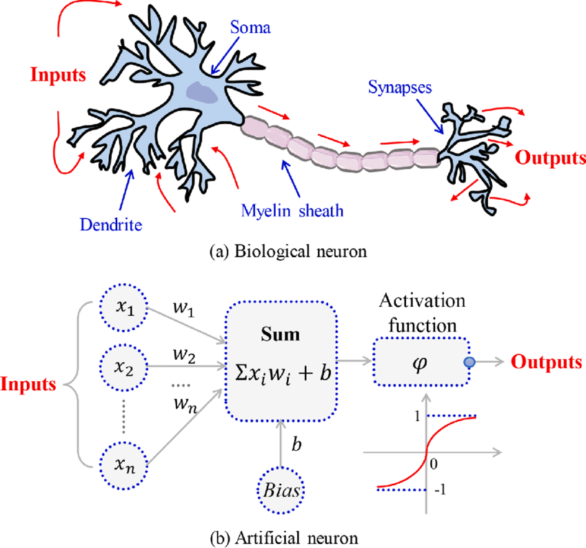
Artificial Neuron
With all these ideas in mind we can now define an Artificial Neuron as a computational unit that :
takes as input \(x=(x_0,x_1,x_2,x_3),\ (x_0 = +1 \equiv bias)\),
outputs \(h_{\theta}(x) = f(\theta^\intercal x) = f(\sum_i \theta_ix_i)\),
where \(f:\mathbb{R}\mapsto \mathbb{R}\) is called the activation function.
Activation functions
Goal of activation function is to provide the neuron with the capability of producing the required outputs.
Flexible enough to produce
- Either linear or non-linear transformations.
- Output in the desired range ([0,1], {-1,1}, \(\mathbb{R}^+\)…)
Usually chosen from a (small) set of possibilities.
- Sigmoid function
- Hyperbolic tangent, or
tanh, function - ReLU
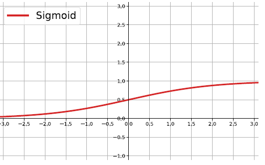
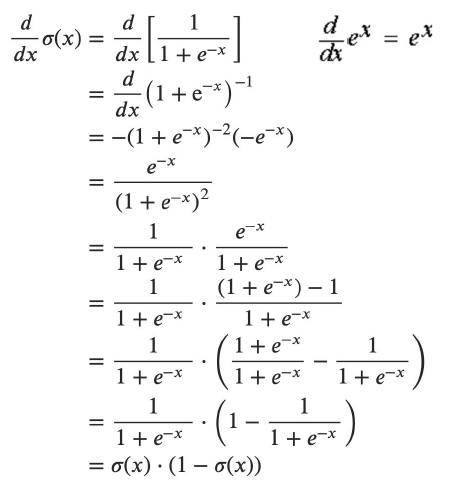
The sigmoid function
\[ f(z)=\frac{1}{1+e^{-z}} \]
Output real values \(\in (0,1)\).
Natural interpretations as probability
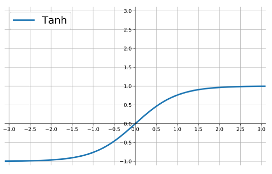
the hyperbolic tangent
Also called tanh, function:
\[ f(z)=\frac{e^{z}-e^{-z}}{e^{z}+e^{-z}} \]
outputs are zero-centered and bounded in −1,1
scaled and shifted Sigmoid
stronger gradient but still has vanishing gradient problem
Its derivative is \(f'(z)=1-(f(z))^2\).
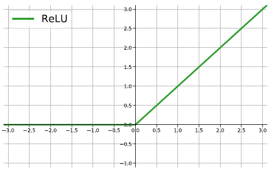
The ReLU
rectified linear unit: \(f(z)=\max\{0,z\}\).
Close to a linear: piece-wise linear function with two linear pieces.
Outputs are in \((0,\infty)\) , thus not bounded
Half rectified: activation threshold at 0
No vanishing gradient problem
More activation functions
 .
.
Softmax Activation Function
Softmax is an activation function used in the output layer of classification models, especially for multi-class problems.
It converts raw scores (logits) into probabilities, ensuring that \(\sum_{i=1}^{N} P(y_i) = 1\) where \(P(y_i)\) is the predicted probability for class \(i\).
Given an input vector \(z\), Softmax transforms it as: \[ \sigma(z_i) = \frac{e^{z_i}}{\sum_{j=1}^{N} e^{z_j}} \]
- The exponentiation amplifies differences, making the highest value more dominant.
- The normalization ensures that probabilities sum to 1.
The Artificial Neuron in Short
The Artificial Neuron in Short
An AN takes a vector of input values \(x_{1}, \ldots, x_{d}\) and combines it with some weights that are local to the neuron \(\left(w_{0}, w_{1}, . ., w_{d}\right)\) to compute a net input \(w_{0}+\sum_{i=1}^{d} w_{i} \cdot x_{i}\).
To compute its output, it then passes the net input through a possibly non-linear univariate activation function \(g(\cdot)\), usually chosen from a set of options such as Sigmoid, Tanh or ReLU functions
To deal with the bias, we create an extra input variable \(x_{0}\) with value always equal to 1 , and so the function computed by a single artificial neuron (parameterized by its weights \(\mathbf{w}\) ) is:
\[ y(\mathbf{x})=g\left(w_{0}+\sum_{i=1}^{d} w_{i} x_{i}\right)=g\left(\sum_{i=0}^{d} w_{i} x_{i}\right)=g\left(\mathbf{w}^{\mathbf{T}} \mathbf{x}\right) \]
From neurons to neural networks
The basic neural network
Continuing with the brain analogy one can combine (artificial) neurons to create better learners.
A simple artificial neural network is created by two types of modifications to the basic Artificial Neuron.
Stacking several neurons insteads of just one.
Adding an additional layer of neurons, which is call a hidden layer,
This yields a system where the output of a neuron can be the input of another in many different ways.
An Artificial Neural network
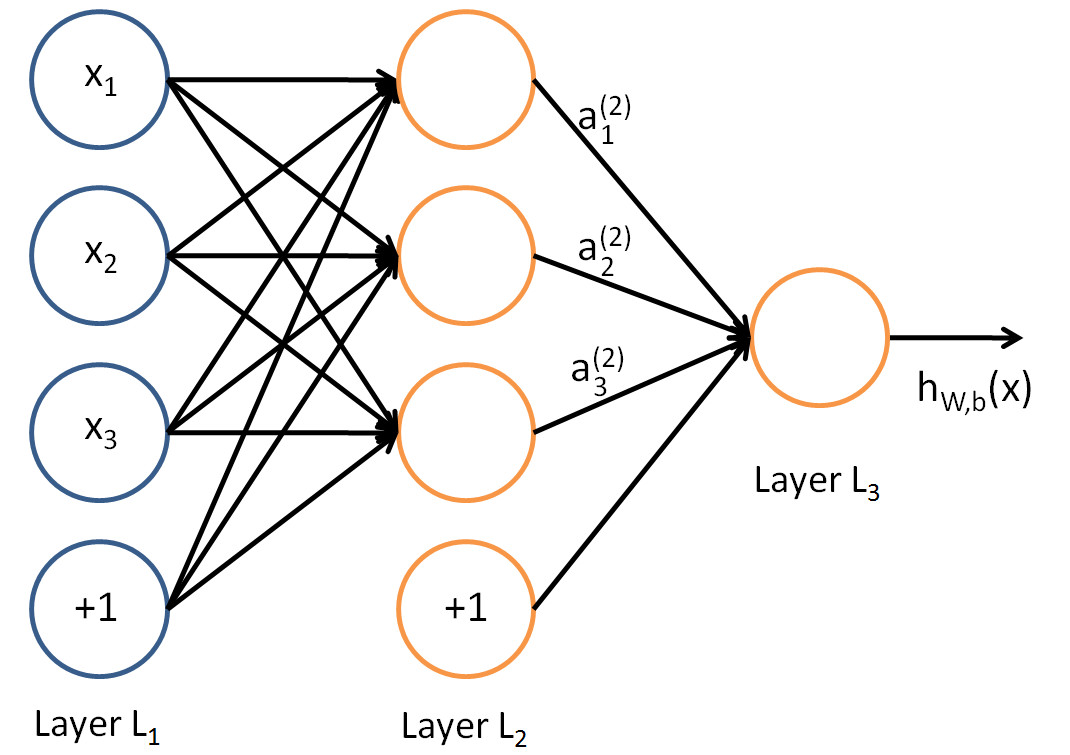
The architecture of ANN
In this figure, we have used circles to also denote the inputs to the network.
Circles labeled +1 are bias units, and correspond to the intercept term.
The leftmost layer of the network is called the input layer.
The rightmost layer of the network is called the output layer.
The middle layer of nodes is called the hidden layer, because its values are not observed in the training set.
Bias nodes are not counted when stating the neuron size.
With all this in mind our example neural network has three layers with:
- 3 input units (not counting the bias unit),
- 3 hidden units,
- 1 output unit.
How an ANN works
An ANN is a predictive model (a learner) whose properties and behaviour can be well characterized.
It operates through a process known as forward propagation, which encompasses the information flow from the input layer to the output layer.
Forward propagation is performed by composing a series of linear and non-linear (activation) functions.
These are characterized (parametrized) by their weights and biases, that need to be learned from data.
- This is done by training the ANN.
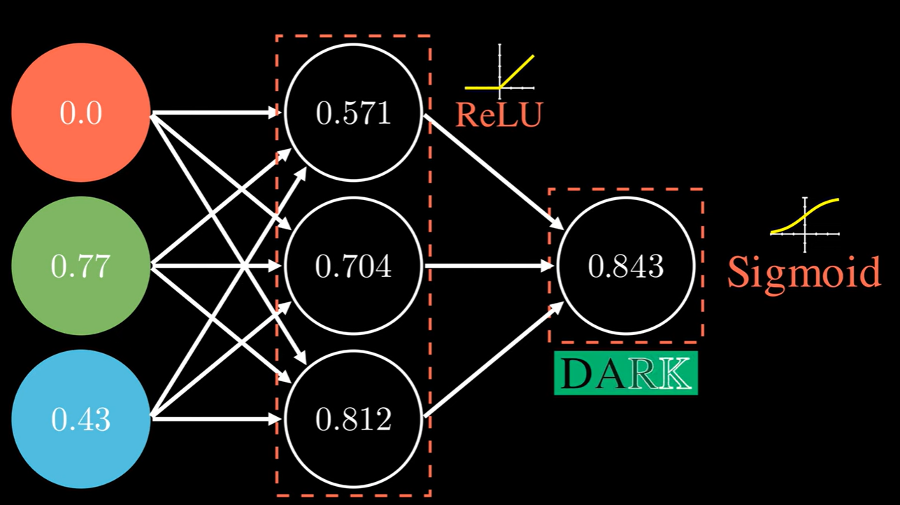
Forward propagation (1)
The process that encompasses the computations required to go from the input values to the final output is known as forward propagation.
For the ANN with 3 input values and 3 neurons in the hidden layer we have:
- Each node \(a_i^{(2)}\) of the hidden layer operates on all input values:
\[\begin{eqnarray} a_1^{(2)}&=&f(\theta_{10}^{(1)}+\theta_{11}^{(1)}x_1+\theta_{12}^{(1)}x_2+\theta_{13}^{(1)}x_3)\\ a_2^{(2)}&=&f(\theta_{20}^{(1)}+\theta_{21}^{(1)}x_1+\theta_{22}^{(1)}x_2+\theta_{23}^{(1)}x_3)\\ a_3^{(2)}&=&f(\theta_{30}^{(1)}+\theta_{31}^{(1)}x_1+\theta_{32}^{(1)}x_2+\theta_{33}^{(1)}x_3) \end{eqnarray}\]
- Output layer: \[ h_{\Theta}(x)=a_1^{(3)}=f(\theta_{10}^{(2)}+\theta_{11}^{(2)}a_1^{(2)}+\theta_{12}^{(2)}a_2^{(2)}+\theta_{13}^{(2)}a_3^{(2)}) \] The terms \(\theta_{i0}^{(l)}\) act as bias parameters.
Forward Propagation (2)
Forward propagation can be written compactly as:
\[ z^{(l+1)} = W^{(l)} a^{(l)} + b^{(l)} \]
\[ a^{(l+1)} = f(z^{(l+1)}) \]
where:
\(W^{(l)}\) contains the weights,
\(b^{(l)}\) contains the bias terms,
\(f(\cdot)\) is applied elementwise.
This form is used in most implementations.
Forward Propagation (3)
An alternative compact notation incorporates the bias into the weight matrix.
Standard form (explicit bias)
\[ z^{(l+1)} = W^{(l)} a^{(l)} + b^{(l)} \]
\[ a^{(l+1)} = f(z^{(l+1)}) \]
- \(W^{(l)}\): weights
- \(b^{(l)}\): bias
- \(f(\cdot)\): elementwise
Augmented form (bias included)
\[ z^{(l+1)} = \Theta^{(l)} \tilde{a}^{(l)} \]
\[ \tilde{a}^{(l)} = \begin{bmatrix} 1 \\ a^{(l)} \end{bmatrix} \]
\[ a^{(l+1)} = f(z^{(l+1)}) \]
- \(\Theta^{(l)} = [\, b^{(l)} \;\; W^{(l)} \,]\)
ANNs as Compositions
In short, a neural network defines a parametric function:
\[ \hat{y} = f(x; \theta) \]
where \(f(\cdot)\) is obtained by composing a sequence of transformations:
\[ f(x) = f^{(L)} \circ f^{(L-1)} \circ \cdots \circ f^{(1)}(x) \]
Each layer defines a transformation of the form:
\[ f^{(l)}(a) = f\big(W^{(l)} a + b^{(l)}\big) \]
so that the activations propagate as:
\[ a^{(l+1)} = f^{(l)}(a^{(l)}) \]
with: \(a^{(1)} = x\) (input layer) and \(a^{(L)} = \hat{y}\) (output layer).
A simple Neural Network
Feed Forward NNs
- The type of NN described is called feed-forward neural network (FFNN), since
- All computations are done by Forward propagation
- The connectivity graph does not have any directed loops or cycles.
Eficient Forward propagation
The way input data is transformed, through a series of weightings and transformations, until the ouput layer is called forward propagation.
By organizing parameters in matrices, and using matrix-vector operations, fast linear algebra routines can be used to perform the required calculations in a fast efficent way.
Multiple architectures for ANN
We have so far focused on a single hidden layer neural network of the example.
One can. however build neural networks with many distinct architectures (meaning patterns of connectivity between neurons), including ones with multiple hidden layers.
Training Neural Networks
Training an ANN
An ANN is a predictive model whose properties and behaviour can be mathematically characterized.
The ANN acts by composing a series of linear and non-linear (activation) functions.
These transformations are characterized by their weights and biases, which need to be learned from data.
Training the network consists in adjusting these parameters so that predictions match -as best as possible- the observed outputs.
Training an ANN
Measuring Prediction Error
To learn the parameters, we need to measure how good the predictions are.
For a given observation \((x, y)\), we use a loss function, \(\ell(y, \hat{y})\) to compare:
- the true output \(y\)
- the predicted output \(\hat{y} = f(x;\theta)\)
Given a dataset \(\{(x_i,y_i)\}_{i=1}^n\), we define the average loss:
\[ J(\theta) = \frac{1}{n} \sum_{i=1}^n \ell(y_i, \hat{y}_i) \]
- This quantity measures how well the network fits the data.
- \(J(\theta)\) is called the cost (or objective) function.
Typical Loss Functions
The choice of loss function depends on the type of problem.
For regression problems a common choice is the squared error: \[ \ell(y, \hat{y}) = (y - \hat{y})^2 \]
For classification problems, we often use loss functions based on probabilities. In particular:
- For binary classification: cross-entropy
- multiclass classification: softmax + cross-entropy
The loss function should reflect how we measure prediction quality.
Cross-entropy loss function
- A common loss function to use with ANNs is Cross-entropy defined as:
\[ l(h_\theta(x),y)=\big{\{}\begin{array}{ll} -\log h_\theta(x) & \textrm{if }y=1\\ -\log(1-h_\theta(x))& \textrm{if }y=0 \end{array} \]
- This function can also be written as:
\[ l(h_\theta(x),y)=-y\log h_\theta(x) - (1-y)\log(1-h_\theta(x)) \]
- Using cross-entropy loss, the cost function is of the form:
\[ J(\theta)=-\frac{1}{n}\left[\sum_{i=1}^n (y^{(i)}\log h_\theta(x^{(i)})+ (1-y^{(i)})\log(1-h_\theta(x^{(i)}))\right] \]
- Now, this is a convex optimization problem.
A probabilistic interpretation
- In binary classification, the network output can be interpreted as a probability:
\[ \hat{y} \approx P(y = 1 \mid x) \]
- Under this interpretation, we associate the model:
\[ P(y \mid x) = \hat{y}^y (1 - \hat{y})^{1-y} \]
- If \(y = 1\), the model assigns probability \(\hat{y}\)
- If \(y = 0\), the model assigns probability \(1 - \hat{y}\)
This probabilistic view is not required, but provides a useful way to motivate the choice of loss function.
A probabilistic interpretation
Given a dataset \(\{(x_i, y_i)\}_{i=1}^n\), we can measure how well the model fits the data (how likely is the model given the data) through the likelihood: \[ L(\theta) = \prod_{i=1}^n \hat{y}_i^{y_i} (1 - \hat{y}_i)^{1-y_i} \]
Maximizing this likelihood is equivalent to minimizing \(- \log L(\theta)\), which leads to the cross-entropy loss: \[ \ell(y, \hat{y}) = -y \log(\hat{y}) - (1 - y)\log(1 - \hat{y}) \] Which should provide a better intuition for this loss function.
From Cost to Optimization
- We have defined a cost function:
\[ J(\theta) = \frac{1}{n} \sum_{i=1}^n \ell(y_i, \hat{y}_i) \]
which measures how well the network fits the data.
- The parameters of the model are:
\[ \theta = \{W^{(l)}, b^{(l)}\}_{l=1}^{L} \]
The key question is: How should we adjust \(\theta\) to reduce \(J(\theta)\)?
Training a network consists in finding the parameters (weights and biases) that minimize the cost function \(J(\theta)\).
Gradient of the Cost Function
The cost function, \(J(\theta)\), depends on all model parameters.
To reduce it, we need to understand how it changes when we modify \(\theta\).
- This is reflected by the derivative or gradient of the function.
The gradient of \(J\) is a vector of partial derivatives defined as:
\[ \nabla J(\theta) = \left( \frac{\partial J}{\partial \theta_1}, \dots, \frac{\partial J}{\partial \theta_p} \right) \]
It indicates how \(J(\theta)\) changes with each parameter.
The gradient vector points in the direction of steepest increase so:
To reduce the cost, we move in the direction of steepest decrease, given by \[-\nabla J(\theta)\]
Gradient Descent Algorithm
To minimize a cost function \(J(\theta)\), we proceeds as follows:
- Initialize \(\theta_0\) randomly or with some predetermined values
- Repeat until convergence: \[ \theta_{t+1} = \theta_{t} - \eta \nabla J(\theta_{t}) \]
- Stop when: \(|J(\theta_{t+1}) - J(\theta_{t})| < \epsilon\)
- \(\theta_0\) is the initial parameter vector,
- \(\theta_t\) is the parameter vector at iteration \(t\),
- \(\eta\) is the learning rate, a step size controlling how large each update is.
- \(\nabla J(\theta_{t})\) is the gradient of the loss function with respect to \(\theta\) at iteration \(t\),
- \(\epsilon\) is a small positive value indicating the desired level of convergence.
Gradient descent Illustration
- Gradient descent is an intuitive approach that has been thoroughly illustrated in many different ways:
https://assets.yihui.org/figures/animation/example/grad-desc
Computing Gradients:
To apply gradient descent, we need to compute \(\nabla J(\theta)\).
The cost depends on the parameters through multiple layers: \[ x \rightarrow a^{(2)} \rightarrow a^{(3)} \rightarrow \cdots \rightarrow \hat{y} \]
Therefore, we must compute derivatives through a composition of functions
Backpropagation, an algorithm introduced in the 1970s in an MSc thesis applies the chain rule to compute these derivatives efficiently
- In 1986, Rumelhart, Hinton, and Williams demonstrated that backpropagation significantly improves learning speed.
This enabled neural networks to solve previously intractable problems.
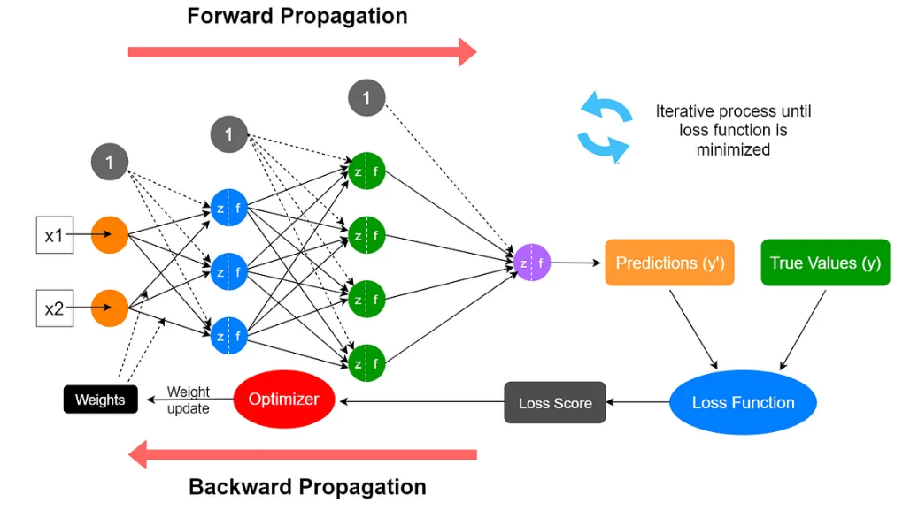
Backpropagation intuition
- The term originates from error backpropagation.
- An artificial neural network computes outputs through forward propagation:
- Input values pass through linear and non-linear transformations.
- The network produces a prediction.
- The error (difference between predicted and true value) is:
- Propagated backward to compute the error contribution of each neuron.
- Used to adjust weights iteratively.
Backpropagation Notation
- For each layer, define:
\[ z^{(l)} = W^{(l-1)} a^{(l-1)} + b^{(l-1)} \]
\[ a^{(l)} = f(z^{(l)}) \]
- Define:
\[ \delta^{(l)} = \frac{\partial J}{\partial z^{(l)}} \]
- \(\delta^{(l)}\) measures how the cost changes with respect to the pre-activation
Output Layer
Recall: \(\delta^{(L)} = \frac{\partial J}{\partial z^{(L)}}\)
The cost depends on \(z^{(L)}\) through the activation \(a^{(L)}\)
Applying the chain rule:
\[ \delta^{(L)} = \frac{\partial J}{\partial a^{(L)}} \odot f'(z^{(L)}) \]
- This term depends on:
- the loss function
- the activation function
- the loss function
Hidden Layers
- The effect of \(z^{(l)}\) on the cost is transmitted through the subsequent layers:
\[ z^{(l)} \rightarrow a^{(l)} \rightarrow z^{(l+1)} \rightarrow J \]
- Applying the chain rule:
\[ \delta^{(l)} = (W^{(l)})^T \delta^{(l+1)} \odot f'(z^{(l)}) \]
The term \((W^{(l)})^T \delta^{(l+1)}\) propagates the effect of the cost backwards
The term \(f'(z^{(l)})\) accounts for the activation function
Forward vs Backward
- Forward propagation:
- computes values
- propagates activations layer by layer
- computes values
\[ x \rightarrow a^{(2)} \rightarrow a^{(3)} \rightarrow \cdots \rightarrow \hat{y} \]
- Backward propagation:
- computes derivatives
- propagates sensitivities (errors) backwards
- computes derivatives
\[ J \rightarrow \delta^{(L)} \rightarrow \delta^{(L-1)} \rightarrow \cdots \rightarrow \delta^{(1)} \]
Forward: how the network produces predictions
Backward: how each parameter affects the cost
Gradients
After propagating the derivatives backwards, we can compute the gradients with respect to the model parameters
Using the chain rule:
\[ \frac{\partial J}{\partial W^{(l)}} = \delta^{(l+1)} (a^{(l)})^T \]
\[ \frac{\partial J}{\partial b^{(l)}} = \delta^{(l+1)} \]
- These expressions follow directly from the definition of \(\delta^{(l)}\)
Backpropagation Summary
- Forward pass:
- compute activations layer by layer
- Backward pass:
- propagate derivatives using the chain rule
- Gradient computation:
- obtain derivatives with respect to all parameters
- Parameter update:
- apply gradient descent
- Backpropagation efficiently computes the gradient \(\nabla J(\theta)\)
A Key Result (1)
- Consider binary classification with:
sigmoid activation
cross-entropy loss
Output layer: \(a^{(L)} = \hat{y} = \sigma(z^{(L)})\)
Loss: \(\ell(y,\hat{y}) = -y \log(\hat{y}) - (1-y)\log(1-\hat{y})\)
- Using the chain rule:
\[ \delta^{(L)} = \frac{\partial J}{\partial z^{(L)}} = \frac{\partial J}{\partial a^{(L)}} \cdot \frac{\partial a^{(L)}}{\partial z^{(L)}} \]
A Key Result (2)
- Computing the derivatives:
\[ \frac{\partial J}{\partial a^{(L)}} = -\frac{y}{\hat{y}} + \frac{1-y}{1-\hat{y}} \]
\[ \frac{\partial a^{(L)}}{\partial z^{(L)}} = \hat{y}(1-\hat{y}) \]
- Combining terms:
\[ \delta^{(L)} = \hat{y} - y \]
- This simple expression greatly simplifies backpropagation
Automatic differentiation
Modern deep learning frameworks do not compute gradients manually.
Instead, they use automatic differentiation and computational graphs to simplify and speed up backpropagation.
A computational graph represents the sequence of operations in a neural network as a directed graph.
- Each node corresponds to an operation (e.g., addition, multiplication, activation function).
- This structure allows efficient backpropagation by applying the chain rule automatically.
Automatic differentiation (AD) relies the computational graph to apply the chain rule and compute gradients automatically in the Backwards pass.
Frameworks like TensorFlow, PyTorch, and JAX use reverse-mode differentiation, which is particularly efficient for functions with many parameters (like neural networks).
Tuning a Neural Network
Improving the learning process
Learning optimization
The learning porocess such as it has been derived may be improved in different ways.
- Predictions can be be bad and require improvement.
- Computations may be inefficent or slow.
- The network may overfit and lack generalizability.
This can be partially soved applying distinct approaches.
Network architechture
Network performance is affected by many hyperparameters
- Network topology
- Number of layers
- Number of neurons per layer
- Activation function(s)
- Weights initialization procedure
- etc.
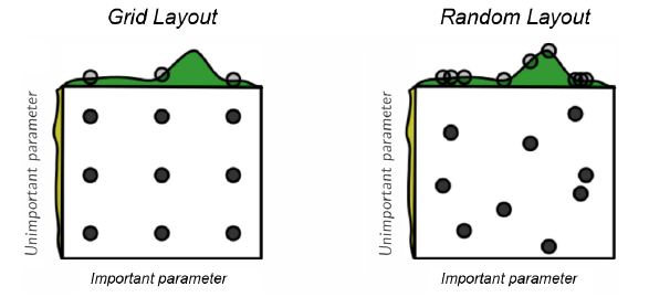
Hyperparameter tuning
- Hyperparameters selection and tuning may be hard, due simply to dimensionality.
- Standard approaches to search for best parameters combinations are used.
How many (hidden) layers
Traditionally considered that one layer may be enough
- Shallow Networks
Posterior research showed that adding more layers increases efficency
- Number of neurons per layer decreases exponentially
Although there is also risk of overfitting
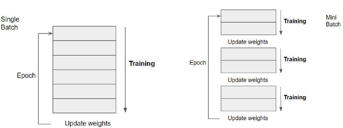
Epochs and iterations
It has been shown that using the whole training set only once may not be enough for training an ANN.
One iteration of the training set is known as an epoch.
The number of epochs \(N_E\), defines how many times we iterate along the whole training set.
\(N_E\) can be fixed, determined by cross-validation or left open and stop the training when it does not improve anymore.
Iterations and batches
A complementary strategy to increasing the number of epochs is decreasing the number of instances in each iteration.
That is, the training set is broken in a number of batches that are trained separately.
Batch learning allows weights to be updated more frequently per epoch.
The advantage of batch learning is related to the gradient descent approach used.
Training in batches
Improving Gradient Descent
- Training deep neural networks involves millions of parameters and large datasets.
- Computing the full gradient in every iteration is computationally expensive because:
- It requires summing over all training points.
- The cost grows linearly with dataset size.
- For large-scale machine learning, standard gradient descent becomes impractical.
- To address this, we use alternative optimization strategies:
- Gradient Descent Variants: Control how much data is used per update.
- Gradient Descent Optimizers: Improve convergence and stability.
Improving Gradient Descent
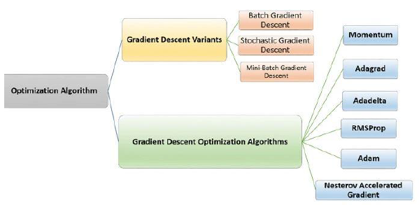
Gradient Descent Variants
- Define how much data is used per update.
- Control the trade-off between computational cost and stability.
- Three common approaches:
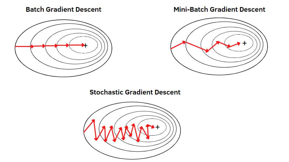
- Batch Gradient Descent:
- Computes the gradient using the entire dataset.
- Stable but slow for large datasets.
- Stochastic Gradient Descent (SGD):
- Computes the gradient using a single training example.
- Faster updates but high variance, leading to noisy convergence.
- Mini-Batch Gradient Descent:
- Uses a subset (mini-batch) of training data per update.
- Balances speed and stability.
- Batch Gradient Descent:
Gradient Descent Variants
Gradient Descent Optimizers
- Improve learning dynamics by modifying how gradients are applied.
- Help avoid local minima, vanishing gradients, and slow convergence.
- Common optimizers:
- Momentum: Uses past gradients to accelerate convergence.
- Adagrad: Adapts the learning rate per parameter.
- Adadelta & RMSProp: Improve Adagrad by reducing aggressive decay.
- Adam: Combines momentum and adaptive learning rates (widely used).
- Nesterov Accelerated Gradient: Improves Momentum with lookahead updates.
Optimizing Training Speed
Training speed can be improved by adjusting key factors that influence convergence.
Weight Initialization: Properly initializing weights helps prevent vanishing or exploding gradients, leading to faster convergence.
Adjusting Learning Rate: A well-tuned learning rate accelerates training while avoiding instability or slow convergence.
Using Efficient Cost Functions: Choosing an appropriate loss function (e.g., cross-entropy for classification) speeds up gradient updates.
Optimizing to Avoid Overfitting
Overfitting occurs when a model learns noise instead of general patterns. Common strategies to prevent it include:
L2 Regularization: Penalizes large weights to reduce model complexity and improve generalization.
Early Stopping: Stops training when validation loss starts increasing, preventing unnecessary overfitting.
Dropout: Randomly disables neurons during training to make the model more robust.
Data Augmentation: Expands the training set by applying transformations (e.g., rotations, scaling) to improve generalization.
Techniques to Improve Training
| Techniques | Performance Improvement | Learning Speed | Overfitting | Description |
|---|---|---|---|---|
| Network Architecture | X | X | X | Adjust layers, neurons andconnections |
| Epochs, Iterations, and Batch Size | X | Controls updates per epoch to improve efficiency. | ||
| Softmax | X | Turns outputs into probabilities | ||
| Training Algorithms | X | X | GD Improvements | |
| Learning Rate | X | X | Step size in gradient updates. | |
| Cross-Entropy Loss | X | Optimized for classification | ||
| L2 Regularization | X | X | Penalizes large weights to prevent overfitting. | |
| Early Stopping | X | Stops training when validation loss worsens. | ||
| Dropout | X | X | Randomly disables neurons to enhance generalization. | |
| Data Augmentation | X | Expands training data by applying transformations. |
Python ANN example
Lab Lab-C3.1-IrisANN-Modular contains a detailed example and a Python notebook on building a NN from scratch.
Lab Lab-C3.1-Dividend Prediction shows how to use R to build and use a Neural network.