
Model validation and Resampling
Alex Sanchez, Ferran Reverter and Esteban Vegas
Genetics Microbiology and Statistics Department. University of Barcelona
Model performance
Assessing model performance
Error estimation and, in general, performance assessment in predictive models is a complex process.
A key challenge is that the true error of a model on new data is typically unknown, and using the training error as a proxy leads to an optimistic evaluation.
Resampling methods, such as cross-validation and the bootstrap, allow us to approximate test error and assess model variability using only the available data.
What is best it can be proven that, well performed, they provide reliable estimates of a model’s performance.
This section introduces these techniques and discusses their practical implications in model assessment.
Prediction (generalization) error
We are interested the prediction or generalization error, the error that will appear when predicting a new observation using a model fitted from some dataset.
Although we don’t know it, it can be estimated using either the training error or the test error estimators.
Training Error vs Test error
The test error is the average error that results from using a statistical learning method to predict the response on a new observation, one that was not used in training the method.
The training error is calculated from the difference among the predictions of a model and the observations used to train it.
Training error rate often is quite different from the test error rate, and in particular the former can dramatically underestimate the latter.
The three errors
Generalization Error. True expected test error (unknown). No bias \[\mathcal{E}(f) = \mathbb{E}_{X_0, Y_0} [ L(Y_0, f(X_0)) ]\]
Test Error Estimator. Estimate of generalization error. Small bias. \[\hat{\mathcal{E}}_{\text{test}}=\frac{1}{m} \sum_{j=1}^{m} L(Y_j^{\text{test}}, f(X_j^{\text{test}}))\]
Training Error Estimator. Measures fit to training data (optimistic). High bias \[\hat{\mathcal{E}}_{\text{train}}: \frac{1}{n} \sum_{i=1}^{n} L(Y_i^{\text{train}}, f(X_i^{\text{train}}))\]
Training- versus Test-Set Performance
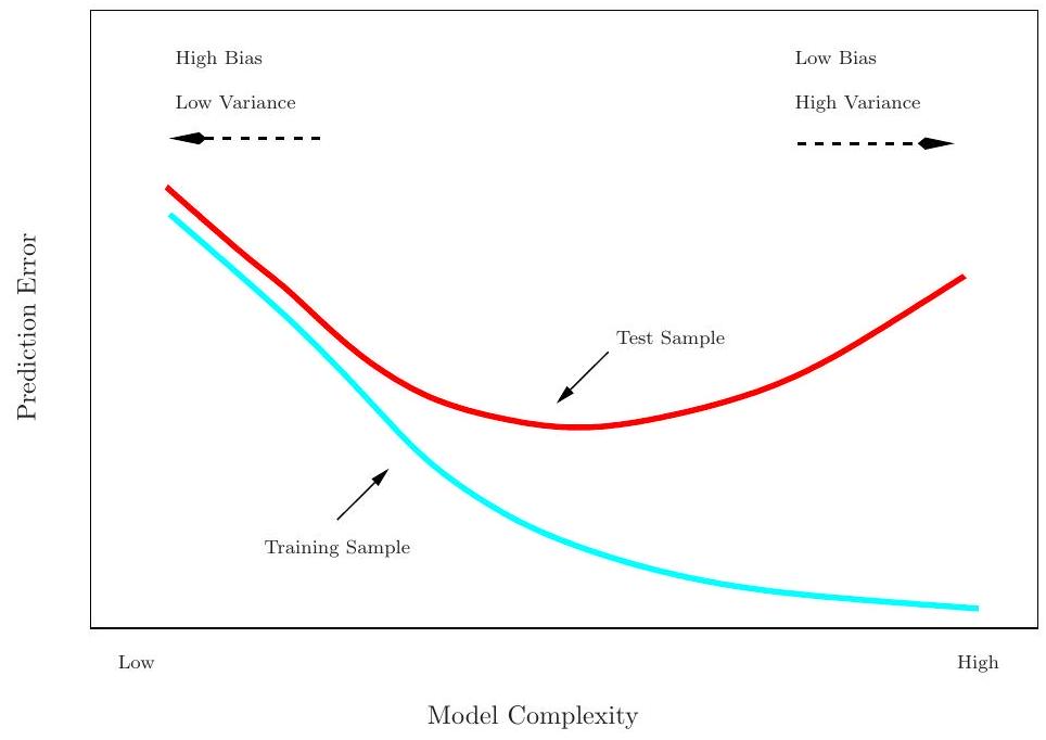
Prediction-error estimates
Ideal: a large designated test set. Often not available
Some methods make a mathematical adjustment to the training error rate in order to estimate the test error rate: \(Cp\) statistic, \(AIC\) and \(BIC\).
Instead, we consider a class of methods that
- Estimate test error by holding out a subset of the training observations from the fitting process, and
- Apply learning method to held out observations
Validation-set approach
Randomly divide the available samples into two parts: a training set and a validation or hold-out set.
The model is fit on the training set, and the fitted model is used to predict the responses for the observations in the validation set.
The resulting validation-set error provides an estimate of the test error. This is assessed using:
- MSE in the case of a quantitative response and
- Misclassification rate in qualitative response.
The Validation process
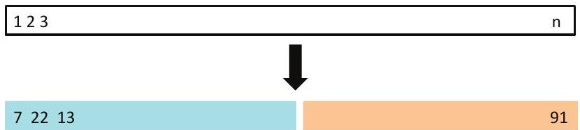
A random splitting into two halves: left part is training set, right part is validation set
Example: automobile data
Goal: compare linear vs higher-order polynomial terms in a linear regression
Method: randomly split the 392 observations into two sets,
- Training set containing 196 of the data points,
- Validation set containing the remaining 196 observations.
Example: automobile data (plot)
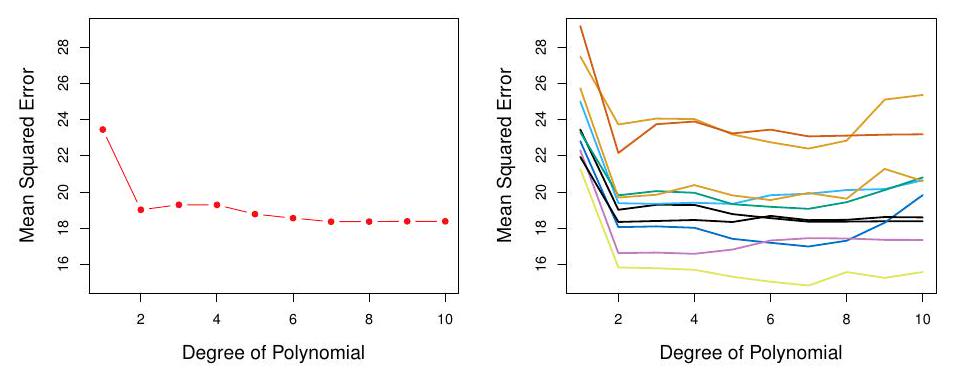
Left panel single split; Right panel shows multiple splits
Drawbacks of the (VS) approach
In the validation approach, only a subset of the observations -those that are included in the training set rather than in the validation set- are used to fit the model.
The validation estimate of the test error can be highly variable, depending on which observations are included in the training set and which are included in the validation set.
This suggests that validation set error may tend to over-estimate the test error for the model fit on the entire data set.
Cross-Validation
\(K\)-fold Cross-validation
Widely used approach for estimating test error.
Estimates give an idea of the test error of the final chosen model
Estimates can be used to select best model,
\(K\)-fold CV mechanism
- Randomly divide the data into \(K\) equal-sized parts.
- Repeat for each part \(k=1,2, \ldots K\),
- Leave one part, \(k\), apart.
- Fit the model to the combined remaining \(K-1\) parts,
- Then obtain predictions for the left-out \(k\)-th part.
- Combine the results to obtain the crossvalidation estimate of tthe error.
\(K\)-fold Cross-validation in detail
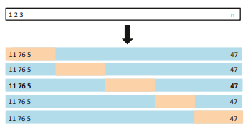
A schematic display of 5-fold CV. A set of n observations is randomly split into fve non-overlapping groups. Each of these ffths acts as a validation set (shown in beige), and the remainder as a training set (shown in blue). The test error is estimated by averaging the fve resulting MSE estimates
The details
Let the \(K\) parts be \(C_{1}, C_{2}, \ldots C_{K}\), where \(C_{k}\) denotes the indices of the observations in part \(k\). There are \(n_{k}\) observations in part \(k\) : if \(N\) is a multiple of \(K\), then \(n_{k}=n / K\).
Compute \[ \mathrm{CV}_{(K)}=\sum_{k=1}^{K} \frac{n_{k}}{n} \mathrm{MSE}_{k} \] where \(\mathrm{MSE}_{k}=\sum_{i \in C_{k}}\left(y_{i}-\hat{y}_{i}\right)^{2} / n_{k}\), and \(\hat{y}_{i}\) is the fit for observation \(i\), obtained from the data with part \(k\) removed.
\(K=n\) yields \(n\)-fold or leave-one out cross-validation (LOOCV).
Auto data revisited
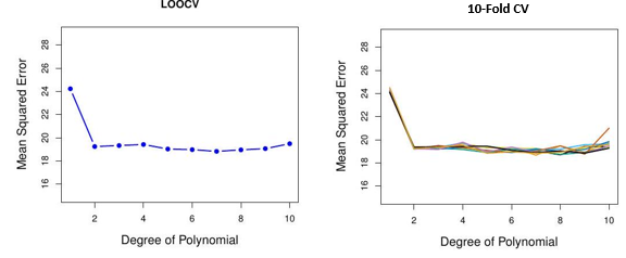
Issues with Cross-validation
- Since each training set is only \((K-1) / K\) as big as the original training set, the estimates of prediction error will typically be biased upward. Why?
- This bias is minimized when \(K=n\) (LOOCV), but this estimate has high variance, as noted earlier.
- \(K=5\) or 10 provides a good compromise for this bias-variance tradeoff.
CV for Classification Problems
- Divide the data into \(K\) roughly equal-sized parts \(C_{1}, C_{2}, \ldots C_{K}\).
- There are \(n_{k}\) observations in part \(k\) and \(n_{k}\simeq n / K\).
- Compute \[ \mathrm{CV}_{K}=\sum_{k=1}^{K} \frac{n_{k}}{n} \operatorname{Err}_{k} \] where \(\operatorname{Err}_{k}=\sum_{i \in C_{k}} I\left(y_{i} \neq \hat{y}_{i}\right) / n_{k}\).
Standard error of CV estimate
- The estimated standard deviation of \(\mathrm{CV}_{K}\) is:
\[ \widehat{\mathrm{SE}}\left(\mathrm{CV}_{K}\right)=\sqrt{\frac{1}{K} \sum_{k=1}^{K} \frac{\left(\operatorname{Err}_{k}-\overline{\operatorname{Err}_{k}}\right)^{2}}{K-1}} \]
- This is a useful estimate, but strictly speaking, not quite valid. Why not?
Why is this an issue?
In (K)-fold CV, the same dataset is used repeatedly for training and testing across different folds.
This introduces correlations between estimated errors in different folds because each fold’s training set overlaps with others.
The assumption underlying this estimation of the standard error is that \(\operatorname{Err}_{k}\) values are independent, which does not hold here.
The dependence between folds leads to underestimation of the true variability in \(\mathrm{CV}_K\), meaning that the reported standard error is likely too small, giving a misleading sense of precision in the estimate of the test error.
CV: right and wrong
Consider a classifier applied to some 2-class data:
- Start with 5000 predictors & 50 samples and find the 100 predictors most correlated with the class labels.
- We then apply a classifier such as logistic regression, using only these 100 predictors.
In order to estimate the test set performance of this classifier, ¿can we apply cross-validation in step 2, forgetting about step 1?
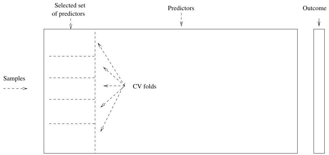
CV the Wrong and the Right way
Applying CV only to Step 2 ignores the fact that in Step 1, the procedure has already used the labels of the training data.
This is a form of training and must be included in the validation process.
- Wrong way: Apply cross-validation in step 2.
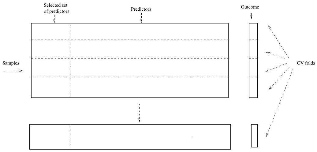
- Right way: Apply cross-validation to steps 1 and 2.
This error has happened in many high profile papers, mainly due to a misunderstanding of what CV means and does.
Wrong Way
Right Way
The Bootstrap
Introducing the Bootstrap
A flexible and powerful statistical tool that can be used to quantify the uncertainty associated with an estimator or a statistical learning method.
It can provide estimates of the standard error or confidence intervals for that estimator/method.
Indeed, it can be applied to any (or most) situations where one needs to deal with variability, that the method can approximate using resampling.
Where does the name came from?
The term derives from the phrase “to pull oneself up by one’s bootstraps”, thought to be based on the XVIIIth century book ” The Surprising Adventures of Baron Munchausen”.
It is not the same as the term “bootstrap” used in computer science meaning to “boot” a computer from a set of core instructions.
Origins of the bootstrap

A simple example
- Suppose that we wish to invest a fixed sum of money in two financial assets that yield returns of \(X\) and \(Y\), respectively, where \(X\) and \(Y\) are random quantities.
- We will invest a fraction \(\alpha\) of our money in \(X\), and will invest the remaining \(1-\alpha\) in \(Y\).
- We wish to choose \(\alpha\) to minimize the total risk, or variance, of our investment. In other words, we want to minimize \(\operatorname{Var}(\alpha X+(1-\alpha) Y)\).
Example continued
The value that minimizes the risk is: \[ \alpha=\frac{\sigma_{Y}^{2}-\sigma_{X Y}}{\sigma_{X}^{2}+\sigma_{Y}^{2}-2 \sigma_{X Y}} \] where:
\(\sigma_{X}^{2}=\operatorname{Var}(X)\)
\(\sigma_{Y}^{2}=\operatorname{Var}(Y)\) and
\(\sigma_{X Y}=\operatorname{Cov}(X, Y)\).
Example continued
- The values of \(\sigma_{X}^{2}, \sigma_{Y}^{2}\), and \(\sigma_{X Y}\) are unknown.
- We can compute estimates for these quantities, \(\hat{\sigma}_{X}^{2}, \hat{\sigma}_{Y}^{2}\), and \(\hat{\sigma}_{X Y}\), using a data set that contains measurements for \(X\) and \(Y\).
- We can then estimate the value of \(\alpha\) that minimizes the variance of our investment using \[ \hat{\alpha}=\frac{\hat{\sigma}_{Y}^{2}-\hat{\sigma}_{X Y}}{\hat{\sigma}_{X}^{2}+\hat{\sigma}_{Y}^{2}-2 \hat{\sigma}_{X Y}} \]
Example continued
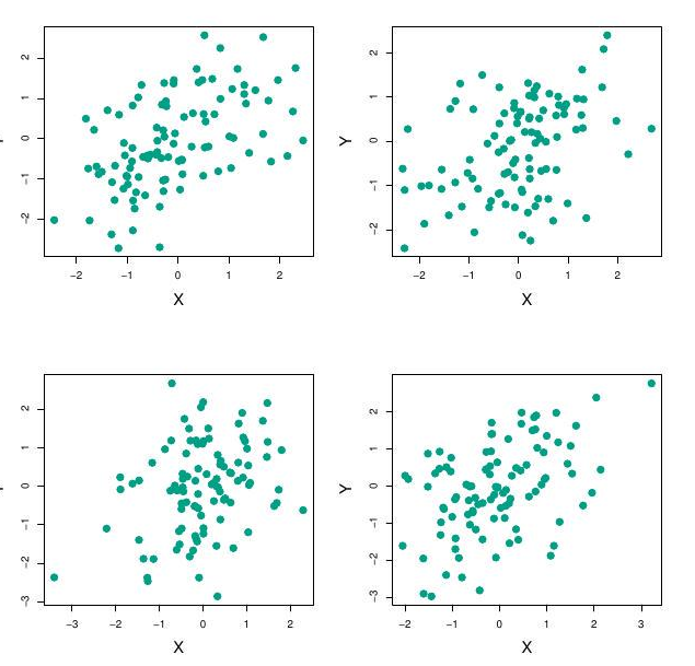
Each panel displays 100 simulated returns for investments \(X\) and \(Y\).
From left to right and top to bottom, the resulting estimates for alpha are
0.576, 0.532, 0.657, and 0.651
Example: How variable is \(\hat \alpha\)?
The standard deviation of \(\hat{\alpha}\), can be estimated as:
- Repeat 1 … 1000 times
- 1.1 Simulate 100 paired observations of \(X\) and \(Y\).
- 1.2 Estimate \(\alpha: \hat{\alpha}_{1}, \hat{\alpha}_{2}, \ldots, \hat{\alpha}_{1000}\).
- Compute the standard deviation of \(\alpha_i\), \(s_{1000}(\hat{\alpha}_i)\) and use it as an estimator of \(SE (\hat{\alpha})\)
- The sample mean of all \(\alpha_i\), \(\overline{\hat{\alpha}_i}\) is also a monte carlo estimate of \(\alpha\), although we are not interested in it.
Example: Simlation results

Left: A histogram of the estimates of \(\alpha\) obtained by generating 1,000 simulated data sets from the true population. Center: A histogram of the estimates of \(\alpha\) obtained from 1,000 bootstrap samples from a single data set. Right: The estimates of \(\alpha\) displayed in the left and center panels are shown as boxplots.
For these simulations the parameters were set to \(\sigma_{X}^{2}=1, \sigma_{Y}^{2}=1.25\), and \(\sigma_{X Y}=0.5\), and so we know that the true value of \(\alpha\) is 0.6 (indicated by the red line).
Example continued
- The mean over all 1,000 estimates for \(\alpha\) is
\[ \bar{\alpha}=\frac{1}{1000} \sum_{r=1}^{1000} \hat{\alpha}_{r}=0.5996,\quad \text { very close to $\alpha=0.6$.} \]
The standard deviation of the estimates computed on the simulated samples: \[ \mathrm{SE}_{Sim}(\hat{\alpha})= \sqrt{\frac{1}{1000-1} \sum_{r=1}^{1000}\left(\hat{\alpha}_{r}-\bar{\alpha}\right)^{2}}=0.083 \]
This gives an idea of the accuracy of \(\hat{\alpha}\) : \(\mathrm{SE}(\hat{\alpha}) \approx \mathrm{SE}_{Sim}(\hat{\alpha})= 0.083\).
So roughly speaking, for a random sample from the population, we would expect \(\hat{\alpha}\) to differ from \(\alpha\) by approximately 0.08 , on average.
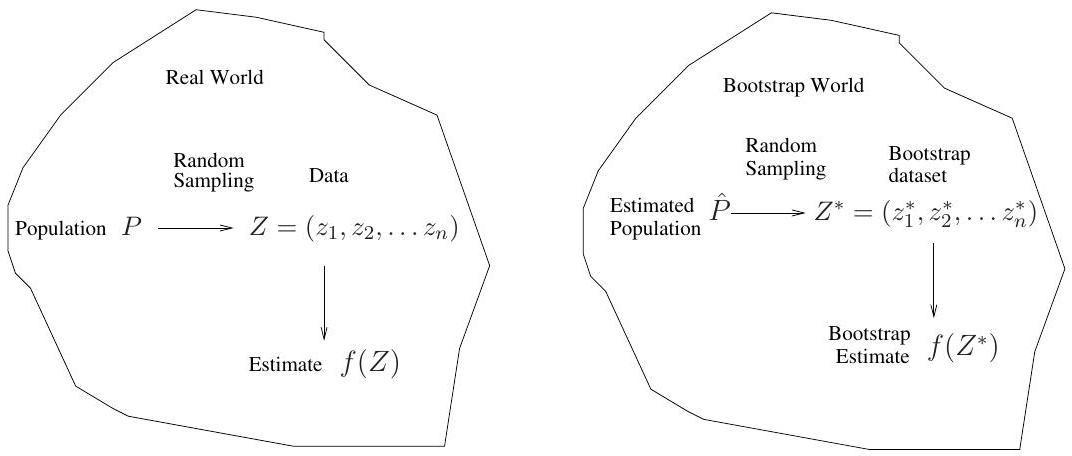
Back to the real world
The procedure outlined above, Monte Carlo Sampling, cannot be applied, because for real data we cannot generate new samples from the original population.
However, the bootstrap approach allows us to use a computer to mimic the process of obtaining new data sets, so that we can estimate the variability of our estimate without generating additional samples.
Sampling the sample = resampling
Rather than repeatedly obtaining independent data sets from the population, we may obtain distinct data sets by repeatedly sampling observations from the original data set with replacement.
This generates a list of “bootstrap data sets” of the same size as our original dataset.
As a result some observations may appear more than once in a given bootstrap data set and some not at all.
Resampling illustrated
Boot. estimate of std error
The standard error of \(\alpha\) can be approximated by the the standard deviation taken on all of these bootstrap estimates using the usual formula: \[ \mathrm{SE}_{B}(\hat{\alpha})=\sqrt{\frac{1}{B-1} \sum_{r=1}^{B}\left(\hat{\alpha}^{* r}-\overline{\hat{\alpha^{*}}}\right)^{2}} \]
This quantity, called bootstrap estimate of standard error serves as an estimate of the standard error of \(\hat{\alpha}\) estimated from the original data set. \[ \mathrm{SE}_{B}(\hat{\alpha}) \approx \mathrm{SE}(\hat{\alpha}) \]
For this example \(\mathrm{SE}_{B}(\hat{\alpha})=0.087\).
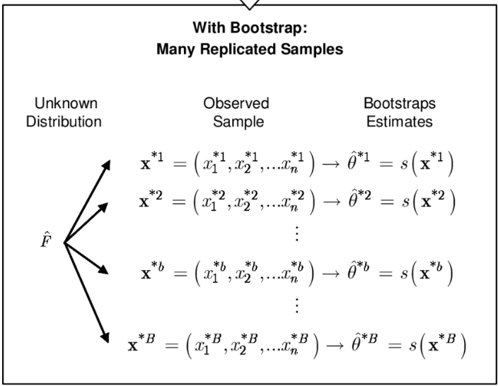
A general picture for the bootstrap
The bootstrap in general
- In more complex data situations, figuring out the appropriate way to generate bootstrap samples can require some thought.
- For example, if the data is a time series, we can’t simply sample the observations with replacement (why not?).
- We can instead create blocks of consecutive observations, and sample those with replacements. Then we paste together sampled blocks to obtain a bootstrap dataset.
Other uses of the bootstrap
- Primarily used to obtain standard errors of an estimate.
- Also provides approximate confidence intervals for a population parameter. For example, looking at the histogram in the middle panel of the Figure on slide 29, the \(5 \%\) and \(95 \%\) quantiles of the 1000 values is (.43, .72 ).
- This represents an approximate \(90 \%\) confidence interval for the true \(\alpha\). How do we interpret this confidence interval?
Other uses of the bootstrap
Primarily used to obtain standard errors of an estimate.
Also provides approximate confidence intervals for a population parameter. For example, looking at the histogram in the middle panel of the Figure on slide 29, the \(5 \%\) and \(95 \%\) quantiles of the 1000 values is (.43, .72 ).
This represents an approximate \(90 \%\) confidence interval for the true \(\alpha\). How do we interpret this confidence interval?
The above interval is called a Bootstrap Percentile confidence interval. It is the simplest method (among many approaches) for obtaining a confidence interval from the bootstrap.
Can the bootstrap estimate prediction error?
In cross-validation, each of the \(K\) validation folds is distinct from the other \(K-1\) folds used for training: there is no overlap. This is crucial for its success. Why?
To estimate prediction error using the bootstrap, we could think about using each bootstrap dataset as our training sample, and the original sample as our validation sample.
But each bootstrap sample has significant overlap with the original data. About two-thirds of the original data points appear in each bootstrap sample. Can you prove this?
This will cause the bootstrap to seriously underestimate the true prediction error. Why?
The other way around- with original sample = training sample, bootstrap dataset \(=\) validation sample - is worse!
Removing the overlap
Can partly fix this problem by only using predictions for those observations that did not (by chance) occur in the current bootstrap sample.
But the method gets complicated, and in the end, cross-validation provides a simpler, more attractive approach for estimating prediction error.
Pre-validation
In microarray and other genomic studies, an important problem is to compare a predictor of disease outcome derived from a large number of “biomarkers” to standard clinical predictors.
Comparing them on the same dataset that was used to derive the biomarker predictor can lead to results strongly biased in favor of the biomarker predictor.
Pre-validation can be used to make a fairer comparison between the two sets of predictors.
Motivating example
An example of this problem arose in the paper of van’t Veer et al. Nature (2002). Their microarray data has 4918 genes measured over 78 cases, taken from a study of breast cancer. There are 44 cases in the good prognosis group and 34 in the poor prognosis group. A “microarray” predictor was constructed as follows:
- 70 genes were selected, having largest absolute correlation with the 78 class labels.
- Using these 70 genes, a nearest-centroid classifier \(C(x)\) was constructed.
- Applying the classifier to the 78 microarrays gave a dichotomous predictor \(z_{i}=C\left(x_{i}\right)\) for each case \(i\).
Results
Comparison of the microarray predictor with some clinical predictors, using logistic regression with outcome prognosis:
| Model | Coef | Stand. Err. | Z score | p-value |
|---|---|---|---|---|
| Re-use | ||||
| microarray | 4.096 | 1.092 | 3.753 | 0.000 |
| angio | 1.208 | 0.816 | 1.482 | 0.069 |
| er | -0.554 | 1.044 | -0.530 | 0.298 |
| grade | -0.697 | 1.003 | -0.695 | 0.243 |
| pr | 1.214 | 1.057 | 1.149 | 0.125 |
| age | -1.593 | 0.911 | -1.748 | 0.040 |
| size | 1.483 | 0.732 | 2.026 | 0.021 |
| Pre-validated | ||||
| microarray | 1.549 | 0.675 | 2.296 | 0.011 |
| angio | 1.589 | 0.682 | 2.329 | 0.010 |
| er | -0.617 | 0.894 | -0.690 | 0.245 |
| grade | 0.719 | 0.720 | 0.999 | 0.159 |
| pr | 0.537 | 0.863 | 0.622 | 0.267 |
| age | -1.471 | 0.701 | -2.099 | 0.018 |
| size | 0.998 | 0.594 | 1.681 | 0.046 |
Idea behind Pre-validation
Designed for comparison of adaptively derived predictors to fixed, pre-defined predictors.
The idea is to form a “pre-validated” version of the adaptive predictor: specifically, a “fairer” version that hasn’t “seen” the response \(y\).
Pre-validation process
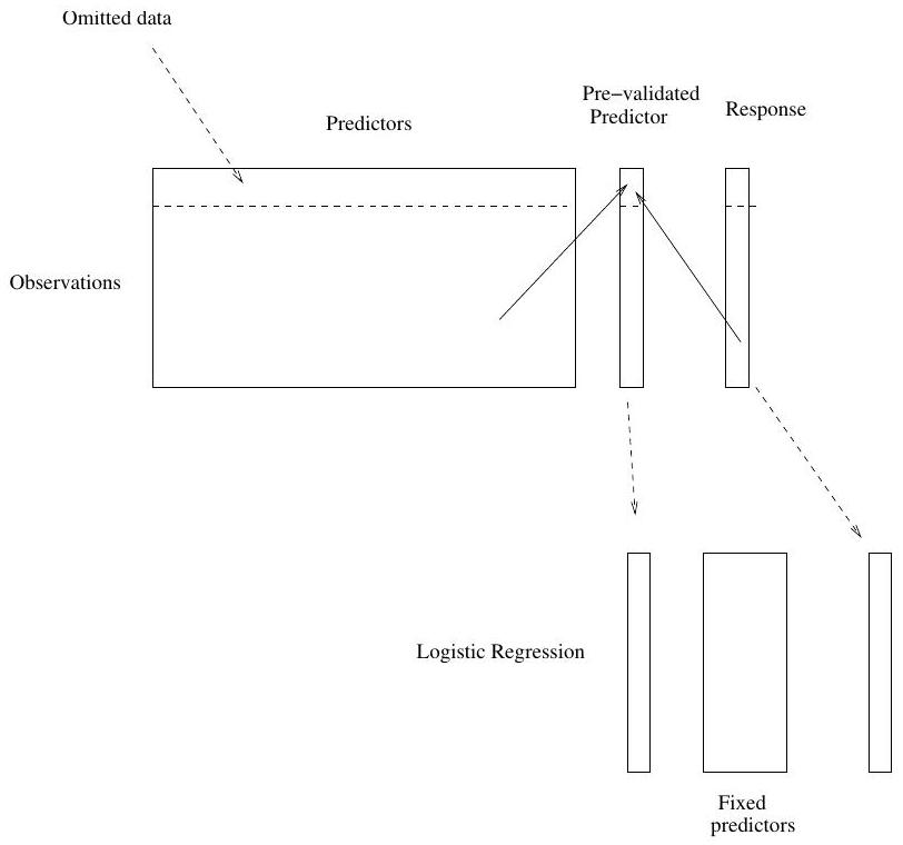
Pre-validation in detail for this example
- Divide the cases up into \(K=13\) equal-sized parts of 6 cases each.
- Set aside one of parts. Using only the data from the other 12 parts, select the features having absolute correlation at least .3 with the class labels, and form a nearest centroid classification rule.
- Use the rule to predict the class labels for the 13th part
- Do steps 2 and 3 for each of the 13 parts, yielding a “pre-validated” microarray predictor \(\tilde{z}_{i}\) for each of the 78 cases.
- Fit a logistic regression model to the pre-validated microarray predictor and the 6 clinical predictors.
The Bootstrap versus Permutation tests
The bootstrap samples from the estimated population, and uses the results to estimate standard errors and confidence intervals.
Permutation methods sample from an estimated null distribution for the data, and use this to estimate p-values and False Discovery Rates for hypothesis tests.
The bootstrap can be used to test a null hypothesis in simple situations. Eg if \(\theta=0\) is the null hypothesis, we check whether the confidence interval for \(\theta\) contains zero.
Can also adapt the bootstrap to sample from a null distribution (See Efron and Tibshirani book “An Introduction to the Bootstrap” (1993), chapter 16) but there’s no real advantage over permutations.