Prediction with (shallow) Neural Networks

Author

Adapted by EVL, FRC and ASP

Published

March 22, 2025

Building a NN with the `neuralnet` package

A predictive ANN

We use the neuralnet package to build a simple neural network to predict if a type of stock pays dividends or not.

Code

if (!require(neuralnet)) 
  install.packages("neuralnet", dep=TRUE)

Data for the example

And use the dividendinfo.csv dataset from https://github.com/MGCodesandStats/datasets

Code

mydata <- read.csv("https://raw.githubusercontent.com/MGCodesandStats/datasets/master/dividendinfo.csv")
str(mydata)

'data.frame':   200 obs. of  6 variables:
 $ dividend       : int  0 1 1 0 1 1 1 0 1 1 ...
 $ fcfps          : num  2.75 4.96 2.78 0.43 2.94 3.9 1.09 2.32 2.5 4.46 ...
 $ earnings_growth: num  -19.25 0.83 1.09 12.97 2.44 ...
 $ de             : num  1.11 1.09 0.19 1.7 1.83 0.46 2.32 3.34 3.15 3.33 ...
 $ mcap           : int  545 630 562 388 684 621 656 351 658 330 ...
 $ current_ratio  : num  0.924 1.469 1.976 1.942 2.487 ...

Data pre-processing

Code

normalize <- function(x) {
  return ((x - min(x)) / (max(x) - min(x)))
}
normData <- as.data.frame(lapply(mydata, normalize))

Test and training sets

Finally we break our data in a test and a training set:

Code

perc2Train <- 2/3
ssize <- nrow(normData)
set.seed(12345)
data_rows <- floor(perc2Train *ssize)
train_indices <- sample(c(1:ssize), data_rows)
trainset <- normData[train_indices,]
testset <- normData[-train_indices,]

Training a neural network

We train a simple NN with two hidden layers, with 4 and 2 neurons respectively.

First we deine the parameters and hyperparameters

Code

hidden_layers <- c(4,2)  # Two hidden layers with 4 and 2 neurons
activation_function <- "logistic"  # Sigmoid
optimizer <- "rprop+"  # Optimizer
learning_rate <- 0.01  # Learning rate
threshold_value <- 0.01  # Convergence  thresholod 
max_iterations <- 1e6  # Max iterations

Code

# Neural Network
library(neuralnet)
nn <- neuralnet(#dividend ~ .,
                dividend ~ fcfps + earnings_growth + de + mcap + current_ratio, 
                data=trainset, 
                hidden=hidden_layers, 
                act.fct=activation_function, 
                algorithm=optimizer, 
                learningrate=learning_rate,
                linear.output=FALSE, 
                threshold=threshold_value,
                stepmax=max_iterations)

Network plot

The output of the procedure is a neural network with estimated weights.

Code

plot(nn, rep = "best")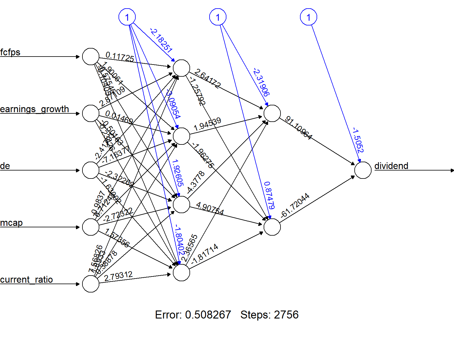

In order to facilitate visualization we can round decimals to 2 for all weights.

Code

round_weights <- function(nn_model, decimals=2) {
  nn_model$weights <- lapply(nn_model$weights, function(layer) {
    lapply(layer, function(weight_matrix) {
      if (is.numeric(weight_matrix)) {
        round(weight_matrix, decimals)
      } else {
        weight_matrix
      }
    })
  })
  return(nn_model)
}

# Apply function to trained net
nn_rounded <- round_weights(nn, 2)

# View network with less decimals
plot(nn_rounded, rep = "best")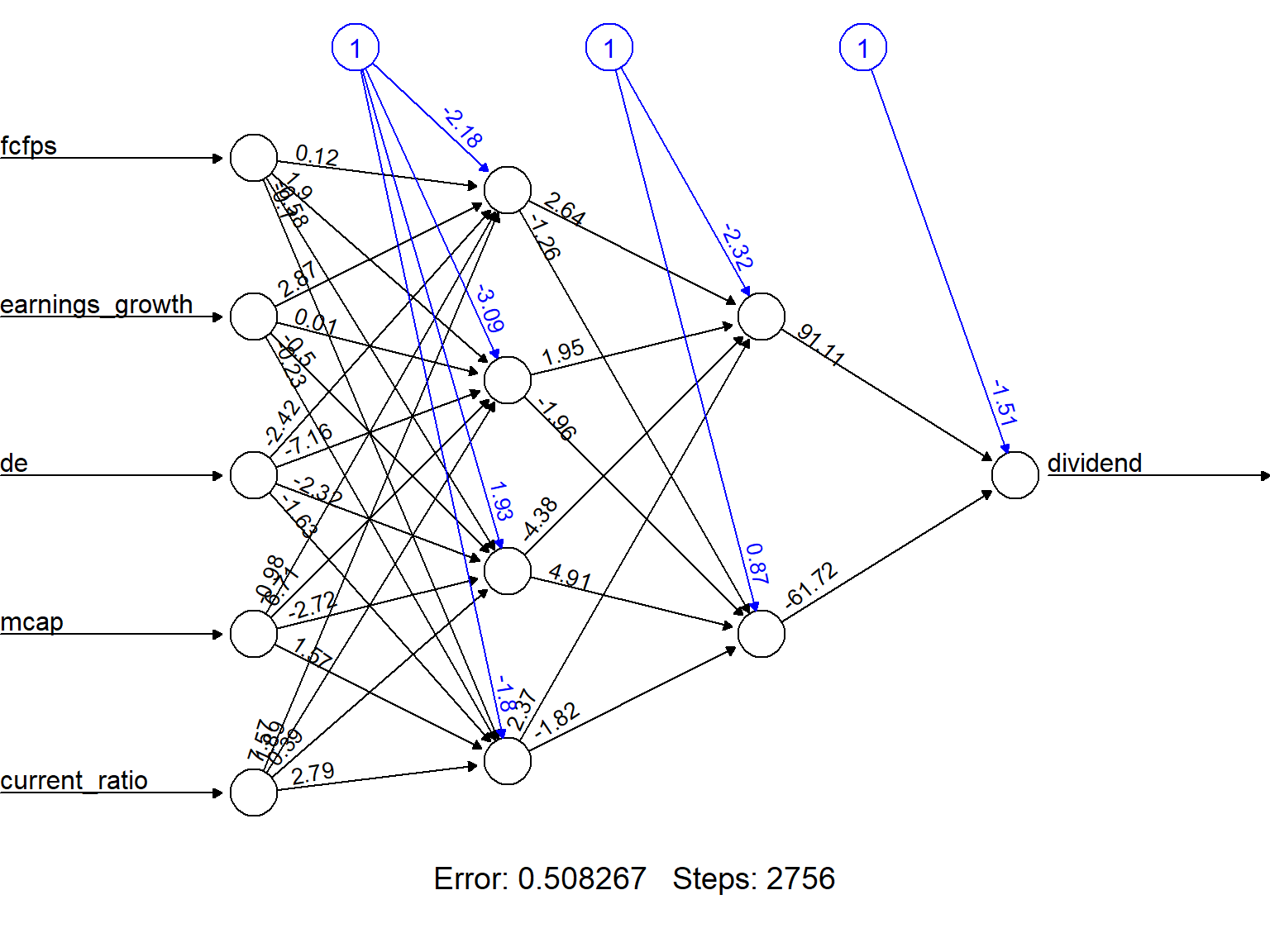

Predictions

Code

temp_test <- subset(testset, select =
                      c("fcfps","earnings_growth", 
                        "de", "mcap", "current_ratio"))
nn.results <- compute(nn, temp_test)
results <- data.frame(actual = 
                  testset$dividend, 
                  prediction = nn.results$net.result)
head(results)

   actual   prediction
9       1 1.000000e+00
19      1 9.999167e-01
22      0 1.184302e-26
26      0 4.282788e-09
27      1 3.686182e-03
29      1 9.999999e-01

Model evaluation

Code

roundedresults<-sapply(results,round,digits=0)
roundedresultsdf=data.frame(roundedresults)
attach(roundedresultsdf)
table(actual,prediction)

      prediction
actual  0  1
     0 35  1
     1  7 24

The caret package can be used to provide a better confusion matrix.

Code

# Round predictions to obtain binary values (0 or 1)
roundedresults <- sapply(results, round, digits=0)
roundedresultsdf <- data.frame(roundedresults)

# Convert variables to factors for proper processing in `caret`
roundedresultsdf$actual <- as.factor(roundedresultsdf$actual)
roundedresultsdf$prediction <- as.factor(roundedresultsdf$prediction)

# Load caret package (install if not available)
if (!require(caret)) install.packages("caret", dependencies=TRUE)
library(caret)

# Generate confusion matrix with advanced metrics
conf_matrix <- confusionMatrix(roundedresultsdf$prediction, roundedresultsdf$actual)

# Print the confusion matrix and performance metrics
print(conf_matrix)

Confusion Matrix and Statistics

          Reference
Prediction  0  1
         0 35  7
         1  1 24
                                         
               Accuracy : 0.8806         
                 95% CI : (0.7782, 0.947)
    No Information Rate : 0.5373         
    P-Value [Acc > NIR] : 1.956e-09      
                                         
                  Kappa : 0.7566         
                                         
 Mcnemar's Test P-Value : 0.0771         
                                         
            Sensitivity : 0.9722         
            Specificity : 0.7742         
         Pos Pred Value : 0.8333         
         Neg Pred Value : 0.9600         
             Prevalence : 0.5373         
         Detection Rate : 0.5224         
   Detection Prevalence : 0.6269         
      Balanced Accuracy : 0.8732         
                                         
       'Positive' Class : 0

Full workflow using `Caret`

The Caret package offers an alternative to neuralnet to perform a more efficient process.

Code

# Load required libraries (install if necessary)
if (!require(caret)) install.packages("caret", dependencies=TRUE)
if (!require(nnet)) install.packages("nnet", dependencies=TRUE)  # Needed for neural networks
library(caret)
library(nnet)

Data can be normalized using using caret’s preProcess function

Code

preproc <- preProcess(mydata, method = c("range"))  # Min-Max normalization
normData <- predict(preproc, mydata)

Test/Train splitting is automated

Code

# Split data into training (67%) and testing (33%) sets
set.seed(12345)
trainIndex <- createDataPartition(normData$dividend, p = 0.67, list = FALSE)
trainset <- normData[trainIndex,]
testset <- normData[-trainIndex,]

Model variability can be managed by crossvalidation

Code

ctrl <- trainControl(method = "cv", number = 10)  # 10-fold cross-validation

Code

# Train a neural network model using caret's `train` function
set.seed(12345)
nn_model <- train(dividend ~ ., data = trainset,
                  method = "nnet",  # Use neural network model
                  trControl = ctrl,  # Cross-validation
                  tuneGrid = expand.grid(size = c(4, 2), decay = 0.01),  # Hidden layers, weight decay
                  maxit = 1000,  # Max iterations
                  trace = FALSE)  # Suppress output during training

# Print model summary
print(nn_model)

Neural Network 

134 samples
  5 predictor

No pre-processing
Resampling: Cross-Validated (10 fold) 
Summary of sample sizes: 120, 120, 121, 121, 120, 120, ... 
Resampling results across tuning parameters:

  size  RMSE       Rsquared   MAE      
  2     0.2009342  0.8309003  0.1048632
  4     0.2007985  0.8313619  0.1021993

Tuning parameter 'decay' was held constant at a value of 0.01
RMSE was used to select the optimal model using the smallest value.
The final values used for the model were size = 4 and decay = 0.01.

Once the model is trained we can proceed as usually

Code

# Make predictions on test set
y_pred <- predict(nn_model, testset)

# Convert predictions to binary (0 or 1)
y_pred_bin <- ifelse(y_pred > 0.5, 1, 0)

# Convert actual values and predictions to factors for confusion matrix
testset$dividend <- as.factor(testset$dividend)
y_pred_bin <- as.factor(y_pred_bin)

# Generate confusion matrix and performance metrics
conf_matrix <- confusionMatrix(y_pred_bin, testset$dividend)

# Print confusion matrix and evaluation metrics
print(conf_matrix)

Confusion Matrix and Statistics

          Reference
Prediction  0  1
         0 34  4
         1  1 27
                                         
               Accuracy : 0.9242         
                 95% CI : (0.832, 0.9749)
    No Information Rate : 0.5303         
    P-Value [Acc > NIR] : 3.522e-12      
                                         
                  Kappa : 0.8471         
                                         
 Mcnemar's Test P-Value : 0.3711         
                                         
            Sensitivity : 0.9714         
            Specificity : 0.8710         
         Pos Pred Value : 0.8947         
         Neg Pred Value : 0.9643         
             Prevalence : 0.5303         
         Detection Rate : 0.5152         
   Detection Prevalence : 0.5758         
      Balanced Accuracy : 0.9212         
                                         
       'Positive' Class : 0

Notice that the model shows slightly better than the first one, probably due to the fact that it has been minimally optimized.

Building a NN with the neuralnet package

A predictive ANN

Data for the example

Data pre-processing

Test and training sets

Training a neural network

Network plot

Predictions

Model evaluation

Full workflow using Caret

Building a NN with the `neuralnet` package

Full workflow using `Caret`