Convolutional Neural Networks

Alex Sanchez, Ferran Reverter and Esteban Vegas

Outline

• Computer Vision and Deep Learning

• Convolutions and Feature Selection

• Convolutional Neural Networks

• A toy example

I. Computer vision and Deep Learning

We want computers that can see

Goal: Computer systems able to see what is present in the world, but also to predict and anticipate events.

source: MIT Course, http://introtodeeplearning.com/, L3

DNN in computer vision systems

Deep Learning enables many systems to undertake a variety of computer vision related tasks.

source: MIT Course, http://introtodeeplearning.com/, L3

Facial detection and recognition

In particular it enables automatic feature extraction.

source: MIT Course, http://introtodeeplearning.com/, L3

Autonomous driving

Autonomus Driving would not be possible without the possibility of performing Automatic Feature Extraction

source: MIT Course, http://introtodeeplearning.com/, L3

Medicine, biology, self care

Neither would systems for automatic disease detection be able to distinguish healthy from affected people though images.

source: MIT Course, http://introtodeeplearning.com/, L3

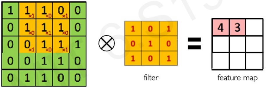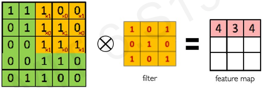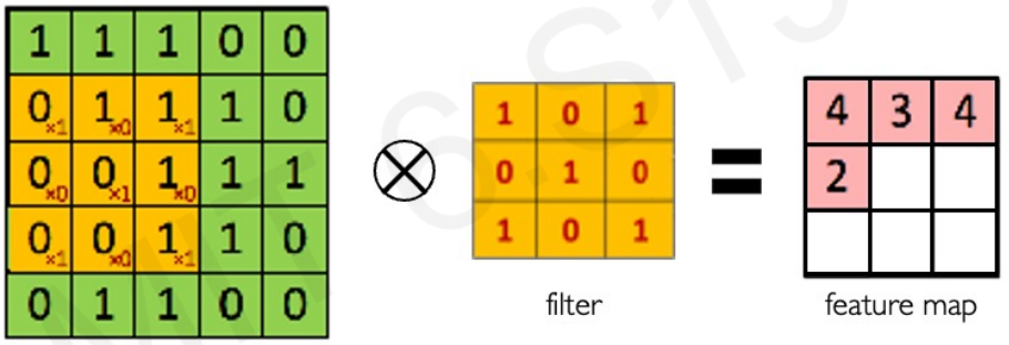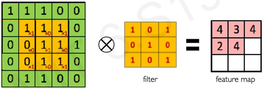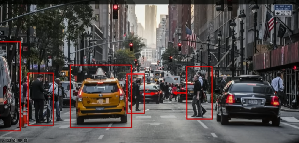
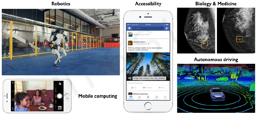
Main tasks in Computer Vision:

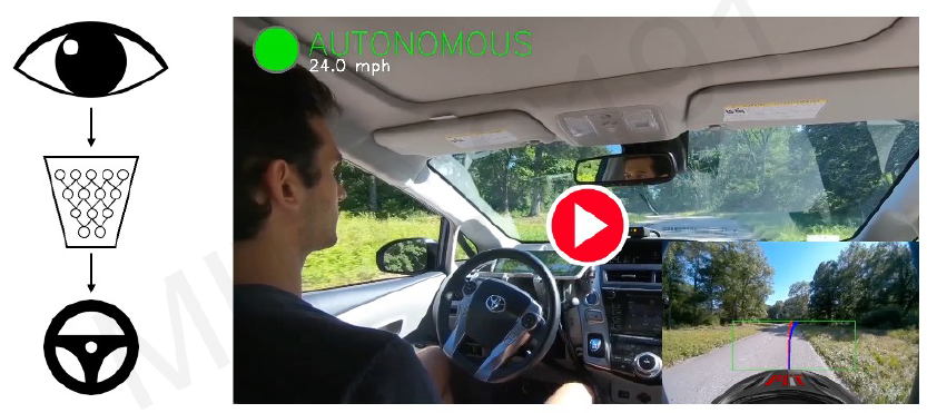
• Regression: Output variable takes continuous value. E.g. Distance to target
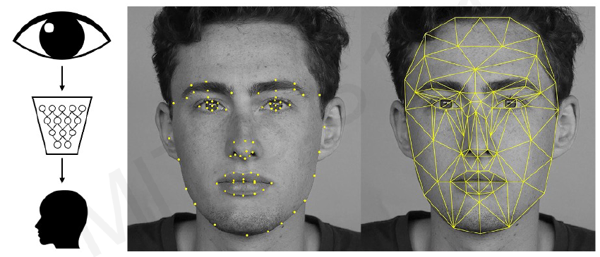
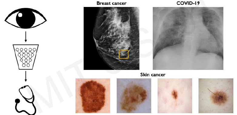
• Classification: Output variable takes class labels. E.g. Probability of belonging to a class

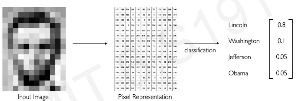
source: MIT Course, http://introtodeeplearning.com/, L3

II. Convolutions and Feature Selection

What (how) do computers see?

• To a computer images, of course, are numbers.

• A greyscale image is a N x M array of numbers.

source: MIT Course, http://introtodeeplearning.com/, L3

What (how) do computers see?

• An RGB (for Red, Green, Blue) color image is an N x M x 3 array of numbers

source: Bhupendra Pratap Singh

High level feature detection

• Each image is characterized by a different set of features.

• Before attempting to build a computer vision system, we need to be aware of what feature keys are in our data that need to be identified and detected.

source: MIT Course, http://introtodeeplearning.com/, L3

How to do feature extraction

• Manual feature extraction is hard!

• Feature characterization needs to define a hierarchy of features allowing an increasing level of detail.

• Deep Neural networks can do this automatically!

source: MIT Course, http://introtodeeplearning.com/, L3

Feature extraction with dense NN

• Fully connected NN could, in principle, be used to learn visual features

source: MIT Course, http://introtodeeplearning.com/, L3

Accounting for spatial structure

• Images have a spatial structure.
• How can this be used to inform the architecture of the Network?

source: MIT Course, http://introtodeeplearning.com/, L3

Extending the idea with patches

source: MIT Course, http://introtodeeplearning.com/, L3

Use filters to extract features

• Filters can be used to extract local features

  • A filter is a set of weights

• Different filters can extract different characteristics.

  • Combining the filters is an efficient way to caracterize an image.

• Filters that matter in one part of the input should matter elsewhere so:

  • Parameters of each filter are spatially shared.

A filter for each pattern?

• By applying different filters, i.e. changing the weights,
• We can achieve completely different results

• In practice filters are combined to completely characterize the images.

Example: “X or X”?

source: MIT Course, http://introtodeeplearning.com/, L3

• Images are represented by matrices of pixels, so
• Literally speaking these images are different.

What are the features of X

• Look for a set of features that:
  • characterize the images, and
  • and are the same in both cases.

source: MIT Course, http://introtodeeplearning.com/, L3

Filters can detect X features

source: MIT Course, http://introtodeeplearning.com/, L3

Is a given pattern in the image?

• Imagine we want to check if a (small) pattern is contained in an (larger) image.

• A slow option is to do a pixel to pixel comparison.

• A better option is to scan the image using an operation known as convolution of the image and the pattern (here called patch, filter or kernel).

• It is faster and allows detecting how well the patch matches different regions in the image.

The Convolution Operation

• Given an input image \(I\) and a filter (kernel) \(K\), the convolution operation is defined as:

  \[ (I * K)(i,j) = \sum_m \sum_n I(i-m, j-n) K(m,n) \]

• Here:

  • \(I(i,j)\) represents the pixel value at position \((i,j)\) in the image.
  • \(K(m,n)\) represents the kernel values.
  • The summation runs over the dimensions of the kernel.
  • The result \((I * K)(i,j)\) gives a new pixel value after applying the filter at that location.

The Convolution Operation

source: MIT Course, http://introtodeeplearning.com/, L3

• Convolution matches the patch and the image by elementwise multiplication, followed by a sum.
• Given the filters used (+1/-1) if there is absolute coincidence, as in the example, all multiplications will yield 1, and the sum will be 9.
• Two completely different patches would add -9.

Visualizing Convolution

• Consider a 3×3 kernel applied to a 5x5 image:

  \[ I = \begin{bmatrix} x_{11} & x_{12} & \dots & x_{15} \\ x_{21} & x_{22} & \dots & x_{25} \\ \dots & \dots & \dots & \dots \\ x_{51} & x_{52} & \dots & x_{55} \end{bmatrix}, \quad K = \begin{bmatrix} 1 & 0 & 0 \\ 0 & 1 & 0 \\ 1 & 0 & 1 \end{bmatrix} \]

• The kernel slides across the image, performing the weighted sum:

  • Multiply corresponding elements.
  • Sum the results.
  • Store in a new matrix (feature map).

Visualizing Convolution

• Suppose we want to compute the convolution of a 5x5 image and a 3x3 filter.

source: MIT Course, http://introtodeeplearning.com/, L3

The Convolution Operation

1. Slide the 3x3 filter over the input image,
2. Elementwise multiply and
3. Add the outputs

source: MIT Course, http://introtodeeplearning.com/, L3

The Convolution Operation

Can filters be learned?

• Different filters can be used to extract different characteristics from the image.
  • Building filters by trial-and-error can be slow.
• If a NN can learn these filters from the data, then
  • They can be used to classify new images.
• This is what Convolutional Neural Networks is about.

III. Convolutional Neural Networks

Convolutional Neural Networks

• CNNs are a type of Deep Neural Network (DNN) that implement the ideas previously introduced.

  • They use convolutions to learn spatial features from input data, such as images or 3D volumes.
  • CNNs are designed to identify increasingly complex traits by concatenating multiple convolutional layers, where each layer learns higher-level features.
  • Convolutional layers are combined with dense layers that perform the final classification using features extracted by the convolutional layers.

Core Concepts for CNNs

• Before diving into CNNs, it is essential to understand key concepts that enable these models to process data effectively.

• Operations that control:

  • How data is fed into the network,
  • How itis processed, and
  • How important features are extracted.

• We’ll cover

  • Padding,
  • Stride,
  • Convolutions over volumes,
  • Pooling

Padding

• Recall the convolution operation

source: DeepLearning.ai

Padding

• In general, a matrix \(n\times n\) convolved with a \(f\times f\) filter \(\longrightarrow n-f+1,n-f+1\) matrix.

• The convolution operation shrinks the matrix if \(f>1\).

• Applying convolution multiple times

  • Shrinks the imaging., loosing data
  • Uses edges pixels less than other pixels in an image.

• To solve these problems we can pad the input image before convolution by adding some rows and columns to it.

Padding

source: Students Notes on CNN

• An appropriate padding, \(p\) avoids the image to shrik.

• Size after convolution: \(n+2p-f+1, n+2p-f+1\).

Strided convolutions

• The cost of convolution can be decreased by increasing step size, \(S\) when moving the filter over the image.

  • In previous examples \(S=1\)
  • See next slide for an example with \(S=2\).

• A matrix nxn convolved with fxf filter and padding p and stride s yields a matrix of size: \[\frac{(n+2p-f)}{s}+1\]

• If (n+2p-f)/s + 1 is fractionary, take floor of this value.

Stride

source: DeepLearning.ai

Convolution over volumes

• On RGB images the filter is a 3-dimensional object.

• We will convolve an image of height \(H_I\), width \(W_I\) and # of channels \(C\), with a filter of height \(H_f\), width \(W_f\) and with same number of channels, \(C\).

• Applying convolution is similar, but at each step,

  • we do \(W_f\times H_f \times C\) multiplications and
  • we sum all the numbers to get 1 output value.

• Sizing formulas above apply because # of channels, \(C\), is not taken into account to determine size of the output.

Convolution over volumes

A convolution with several channels does not increase output dimensions. Source: Students Notes on CNN

Convolution with 2 filters

Multiple filters can be used in a convolution layer to detect multiple features. The output of the layer then will have the same number of channels as the number of filters in the layer..
Source: Students Notes on CNN

One convolutio Layer

• Combining the elements seen above we can build a one layer convolutional network

• It performs the convolution of the input image across all channels nC, uses multiple lters, and therefore originates multiple convolution outputs.

• A bias term b is then added to the output of the convolution of each lter W and we get the equivalent of the term Z in a normal neural network.

• We then apply an activation function such as ReLU Z (on all channels), and we finally stack the channels to create a cube that becomes the network layers output.

One Convolution Layer

Source: Students Notes on CNN

Pooling to decrease dimension

• Additional layers can be added to reduce the size of the representations and so to speed up calculations.

• These are called Pooling Layers

• They have hyper-parameters such as filter size, stride or pooling type.

• But they do not increase the number of parameters: nothing for the gradient descent to learn

Pooling to decrease dimension

source: MIT Course, http://introtodeeplearning.com/, L3

Other benefits of Pooling

Key objectives of pooling in CNNs:

1. Dimensionality Reduction:

2. Translation Invariance:

3. Robustness to Variations:

4. Extraction of Salient Features:

5. Spatial Hierarchy:

Common types of pooling

Source: Students Notes on CNN

• Max pooling: selects the maximum value within each pooling region,
• Average pooling: calculates the average value within each pooling region

A CNN Example: LeNet-5

Source: Students Notes on CNN

• Uses Sigmoid/tanh instead of ReLU
• Average pooling (not max pooling)
• Includes not-linearity after the pooling
• Paper: Gradient-based learning applied to document recognition

Summary: CNNs

• Option of choice for image classification.

• Usually: one or + layers of [convolution + pooling], ended by one or more fully connected layers.

  • Features learned by convolutions
  • Pooling decreases size with spatial invariance

• Usually, input size decreases over layers while the number of filters increases.

• Fully connected layers has the most parameters in the network.

Summary: Why convolutions

CNNs show two main advantages:

• Parameter sharing: A feature detector (e.g. a vertical edge detector) useful in one part of the image is probably useful in another part of the image.

• Sparsity of connections In each layer, each output value depends only on a small number of inputs.

A toy example

The MNIST dataset

• A popular dataset or handwritten numbers.

library(keras)
mnist <- dataset_mnist()

• Made of features (images) and target values (labels)
• Divided into a training and test set.

x_train <- mnist$train$x; y_train <- mnist$train$y
x_test <- mnist$test$x; y_test <- mnist$test$y

(mnistDims <- dim(x_train))
img_rows <- mnistDims[2];  img_cols <- mnistDims[3]

Data pre-processing (1): Reshaping

• These images are not in the the requires shape, as the number of channels is missing.
• This can be corrected using the array_reshape() function.

x_train <- array_reshape(x_train, c(nrow(x_train), img_rows, img_cols, 1))
x_test <- array_reshape(x_test, c(nrow(x_test), img_rows, img_cols, 1)) 

input_shape <- c(img_rows, img_cols, 1)

dim(x_train)

Data pre-processing (2): Other transforms

• Data is first normalized (to values in [0,1])

x_train <- x_train / 255
x_test <- x_test / 255

• Labels are one-hot-encoded using the to_categorical() function.

num_classes = 10
y_train <- to_categorical(y_train, num_classes)
y_test <- to_categorical(y_test, num_classes)

Modeling (1): Definition

model <- keras_model_sequential() %>%
  layer_conv_2d(filters = 16,
                kernel_size = c(3,3),
                activation = 'relu',
                input_shape = input_shape) %>% 
  layer_max_pooling_2d(pool_size = c(2, 2)) %>% 
  layer_dropout(rate = 0.25) %>% 
  layer_flatten() %>% 
  layer_dense(units = 10,
              activation = 'relu') %>% 
  layer_dropout(rate = 0.5) %>% 
  layer_dense(units = num_classes,
              activation = 'softmax')

Modeling (1): Model Summary

model %>% summary()

Modeling (2): Compilation

• Categorical cross-entropy as loss function.
• Adadelta optimizes the gradient descent.
• Accuracy serves as metric.

model %>% compile(
  loss = loss_categorical_crossentropy,
  optimizer = optimizer_adadelta(),
  metrics = c('accuracy')
)

Model training

• A mini-batch¹ size of 128 should allow the tensors to fit into the memory of most “normal” machines.
• The model will run over 12 epochs,
• With a validation split set at 0.2

batch_size <- 128
epochs <- 12

model %>% fit(
  x_train, y_train,
  batch_size = batch_size,
  epochs = epochs,
  validation_split = 0.2
)

1. • A batch is a collection of training examples processed together,
   • A minibatch is a smaller subset of a batch used for memory efficiency
   • An epoch is a complete pass of the entire training dataset during model training.

Model evaluation

• Use test data to evaluate the model.

model %>% evaluate(x_test, y_test)
predictions <- model %>% predict(x_test) # Not shown

References and Resources

Resources (1)

Courses

• An introduction to Deep Learning. Alex Amini. MIT
• Coursera: Deep Learning Specialization. Andrew Ng

Books

• Neural networks and Deep Learning
• Deep learning with R, 2nd edition. F. Chollet

Resources (2)

Workshops

• Deep learning with R Summer course
• Deep learning with keras and Tensorflow in R (Rstudio conf. 2020)

Documents

• Introduction to Convolutional Neural Networks (CNN)
• Convolutional Neural Networks in R