Lab: Decision Trees for Classification and Regression

A guided practical session with questions

Learning goals

This lab is intended to provide an active exercise on classification and regression trees to illustrate how they can be built and used, interpreted and applied.

The main goal is not only to fit a decision tree, but to understand:

1. how a tree partitions the predictor space;
2. how a fitted tree produces class predictions and class probabilities;
3. why training error is not enough to assess prediction performance;
4. how pruning controls model complexity;
5. how the same ideas change when the response is quantitative rather than categorical.

The lab is intentionally written so that most questions are transferable to any similar dataset. The default dataset used here is the Pima Indians diabetes dataset, but the structure can be reused with another classification dataset with minimal changes.

Note on the questions. Questions are numbered automatically using Markdown ordered lists. Some optional questions are kept in the source file as HTML comments. To recover one of them, simply remove the comment delimiters <!-- and -->; the list will be renumbered automatically when the document is rendered.

Packages

packages <- c("mlbench", "rpart", "rpart.plot", "dplyr", "knitr")

for (pkg in packages) {
  if (!require(pkg, character.only = TRUE)) {
    install.packages(pkg)
    library(pkg, character.only = TRUE)
  }
}

Part 1. Classification tree

1.1 Data and prediction problem

In this example we use the PimaIndiansDiabetes2 dataset from the mlbench package.

data("PimaIndiansDiabetes2", package = "mlbench")
mydataset <- PimaIndiansDiabetes2

The response variable is diabetes, a binary factor indicating whether each individual is classified as diabetes-positive or diabetes-negative.

dplyr::glimpse(mydataset)

Rows: 768
Columns: 9
$ pregnant <dbl> 6, 1, 8, 1, 0, 5, 3, 10, 2, 8, 4, 10, 10, 1, 5, 7, 0, 7, 1, 1…
$ glucose  <dbl> 148, 85, 183, 89, 137, 116, 78, 115, 197, 125, 110, 168, 139,…
$ pressure <dbl> 72, 66, 64, 66, 40, 74, 50, NA, 70, 96, 92, 74, 80, 60, 72, N…
$ triceps  <dbl> 35, 29, NA, 23, 35, NA, 32, NA, 45, NA, NA, NA, NA, 23, 19, N…
$ insulin  <dbl> NA, NA, NA, 94, 168, NA, 88, NA, 543, NA, NA, NA, NA, 846, 17…
$ mass     <dbl> 33.6, 26.6, 23.3, 28.1, 43.1, 25.6, 31.0, 35.3, 30.5, NA, 37.…
$ pedigree <dbl> 0.627, 0.351, 0.672, 0.167, 2.288, 0.201, 0.248, 0.134, 0.158…
$ age      <dbl> 50, 31, 32, 21, 33, 30, 26, 29, 53, 54, 30, 34, 57, 59, 51, 3…
$ diabetes <fct> pos, neg, pos, neg, pos, neg, pos, neg, pos, pos, neg, pos, n…

summary(mydataset)

    pregnant         glucose         pressure         triceps     
 Min.   : 0.000   Min.   : 44.0   Min.   : 24.00   Min.   : 7.00  
 1st Qu.: 1.000   1st Qu.: 99.0   1st Qu.: 64.00   1st Qu.:22.00  
 Median : 3.000   Median :117.0   Median : 72.00   Median :29.00  
 Mean   : 3.845   Mean   :121.7   Mean   : 72.41   Mean   :29.15  
 3rd Qu.: 6.000   3rd Qu.:141.0   3rd Qu.: 80.00   3rd Qu.:36.00  
 Max.   :17.000   Max.   :199.0   Max.   :122.00   Max.   :99.00  
                  NA's   :5       NA's   :35       NA's   :227    
    insulin            mass          pedigree           age        diabetes 
 Min.   : 14.00   Min.   :18.20   Min.   :0.0780   Min.   :21.00   neg:500  
 1st Qu.: 76.25   1st Qu.:27.50   1st Qu.:0.2437   1st Qu.:24.00   pos:268  
 Median :125.00   Median :32.30   Median :0.3725   Median :29.00            
 Mean   :155.55   Mean   :32.46   Mean   :0.4719   Mean   :33.24            
 3rd Qu.:190.00   3rd Qu.:36.60   3rd Qu.:0.6262   3rd Qu.:41.00            
 Max.   :846.00   Max.   :67.10   Max.   :2.4200   Max.   :81.00            
 NA's   :374      NA's   :11                                                

Questions

1. What is the response variable? Is this a classification or a regression problem?

2. Identify at least three predictors. For each one, indicate whether it is quantitative or categorical.

3. Before fitting a tree, inspect the data. Are there missing values? If so, in which variables? Why could missing values matter for model fitting and model assessment?

Write your answers here or, if available, in the online form provided for the exercise

1.2 Minimal preprocessing

Given this is a classroom lab, we will remove all missing values and use only complete cases. This is not necessarily the best strategy in a real analysis, but it keeps the focus on tree construction and model assessment.

mydataset_cc <- na.omit(mydataset)

dim(mydataset)

[1] 768   9

dim(mydataset_cc)

[1] 392   9

table(mydataset$diabetes)

neg pos 
500 268 

table(mydataset_cc$diabetes)

neg pos 
262 130 

Questions

1. What is the consequence of using na.omit()? In a real study, what alternative preprocessing strategy could be considered?

Write your answers here or, if available, in the online form provided for the exercise

1.3 Train/test split

We split the dataset into training and test sets. The model will be fitted using the training set and evaluated using the test set.

set.seed(123)

prop_train <- 0.70
n <- nrow(mydataset_cc)
train_id <- sample(seq_len(n), size = floor(prop_train * n))

train_data <- mydataset_cc[train_id, ]
test_data  <- mydataset_cc[-train_id, ]

nrow(train_data)

[1] 274

nrow(test_data)

[1] 118

table(train_data$diabetes)

neg pos 
179  95 

table(test_data$diabetes)

neg pos 
 83  35 

Questions

1. Why do we split the data into training and test sets instead of evaluating the tree on the same data used to fit it?

2. Check whether the class distribution is similar in the training and test sets. Why could a very unbalanced split be problematic?

Write your answers here or, if available, in the online form provided for the exercise.

Part 2. Fitting and interpreting a classification tree

2.1 Fit an initial tree

We fit a classification tree using rpart().

require(rpart)
tree_class <- rpart(
  diabetes ~ ., 
  data = train_data,
  method = "class",
  control = rpart.control(cp = 0.001)
)

tree_class

n= 274 

node), split, n, loss, yval, (yprob)
      * denotes terminal node

 1) root 274 95 neg (0.65328467 0.34671533)  
   2) glucose< 127.5 163 24 neg (0.85276074 0.14723926)  
     4) pedigree< 0.5085 97  4 neg (0.95876289 0.04123711) *
     5) pedigree>=0.5085 66 20 neg (0.69696970 0.30303030)  
      10) age< 27.5 38  4 neg (0.89473684 0.10526316) *
      11) age>=27.5 28 12 pos (0.42857143 0.57142857)  
        22) glucose< 98.5 7  1 neg (0.85714286 0.14285714) *
        23) glucose>=98.5 21  6 pos (0.28571429 0.71428571) *
   3) glucose>=127.5 111 40 pos (0.36036036 0.63963964)  
     6) glucose< 157.5 73 36 pos (0.49315068 0.50684932)  
      12) mass< 30.2 23  5 neg (0.78260870 0.21739130) *
      13) mass>=30.2 50 18 pos (0.36000000 0.64000000)  
        26) pedigree< 0.285 14  5 neg (0.64285714 0.35714286) *
        27) pedigree>=0.285 36  9 pos (0.25000000 0.75000000)  
          54) glucose>=152 8  3 neg (0.62500000 0.37500000) *
          55) glucose< 152 28  4 pos (0.14285714 0.85714286) *
     7) glucose>=157.5 38  4 pos (0.10526316 0.89473684) *

require(rpart.plot)
rpart.plot(tree_class, extra = 104, fallen.leaves = TRUE, cex = 0.7)

The argument extra = 104 displays the predicted class, the class probabilities and the percentage of observations in each node.

Questions

1. Which predictor appears in the root node? What does this suggest about its predictive role in this fitted tree?

2. Choose one internal split. Explain it as a decision rule of the form: “if predictor X is below/above a threshold, then observations go to…”.

1. Explain, in your own words, how the tree transforms a vector of predictors \(x\) into a class prediction \(\hat{y}\).

Write your answers here or, if available, in the online form provided for the exercise.

Adjusting the parameters

If we compare the tree obtained with that produced by using Python version of this lab we see that the second split is different (based on distinct variables).

While the explanantion is not obvious we can force the parameters to make both programs to produce a similar output.

In order to try to reduce differences due to random splitting we build a temporary tree with all data and attempting to pair parameter values among python and R calls.

tree_class_v2 <- rpart(
  diabetes ~ ., 
  data = mydataset_cc,
  method = "class",
  control = rpart.control(
    cp = 0,
    minsplit = 2,
    minbucket = 1,
    maxdepth = 30
  )
)

tree_class_v2

n= 392 

node), split, n, loss, yval, (yprob)
      * denotes terminal node

   1) root 392 130 neg (0.66836735 0.33163265)  
     2) glucose< 127.5 241  36 neg (0.85062241 0.14937759)  
       4) insulin< 143.5 181  16 neg (0.91160221 0.08839779)  
         8) pedigree< 0.4955 113   4 neg (0.96460177 0.03539823)  
          16) mass< 45.35 111   3 neg (0.97297297 0.02702703)  
            32) pregnant< 9.5 107   2 neg (0.98130841 0.01869159)  
              64) pressure>=51 100   1 neg (0.99000000 0.01000000)  
               128) insulin>=36.5 92   0 neg (1.00000000 0.00000000) *
               129) insulin< 36.5 8   1 neg (0.87500000 0.12500000)  
                 258) pressure< 81.5 7   0 neg (1.00000000 0.00000000) *
                 259) pressure>=81.5 1   0 pos (0.00000000 1.00000000) *
              65) pressure< 51 7   1 neg (0.85714286 0.14285714)  
               130) glucose>=85.5 5   0 neg (1.00000000 0.00000000) *
               131) glucose< 85.5 2   1 neg (0.50000000 0.50000000)  
                 262) pregnant< 2 1   0 neg (1.00000000 0.00000000) *
                 263) pregnant>=2 1   0 pos (0.00000000 1.00000000) *
            33) pregnant>=9.5 4   1 neg (0.75000000 0.25000000)  
              66) glucose< 112.5 3   0 neg (1.00000000 0.00000000) *
              67) glucose>=112.5 1   0 pos (0.00000000 1.00000000) *
          17) mass>=45.35 2   1 neg (0.50000000 0.50000000)  
            34) pregnant>=4.5 1   0 neg (1.00000000 0.00000000) *
            35) pregnant< 4.5 1   0 pos (0.00000000 1.00000000) *
         9) pedigree>=0.4955 68  12 neg (0.82352941 0.17647059)  
          18) glucose< 103 49   4 neg (0.91836735 0.08163265)  
            36) mass< 50.9 48   3 neg (0.93750000 0.06250000)  
              72) pedigree< 0.817 34   0 neg (1.00000000 0.00000000) *
              73) pedigree>=0.817 14   3 neg (0.78571429 0.21428571)  
               146) pedigree>=0.894 12   1 neg (0.91666667 0.08333333)  
                 292) glucose>=80.5 10   0 neg (1.00000000 0.00000000) *
                 293) glucose< 80.5 2   1 neg (0.50000000 0.50000000)  
                   586) pregnant< 2 1   0 neg (1.00000000 0.00000000) *
                   587) pregnant>=2 1   0 pos (0.00000000 1.00000000) *
               147) pedigree< 0.894 2   0 pos (0.00000000 1.00000000) *
            37) mass>=50.9 1   0 pos (0.00000000 1.00000000) *
          19) glucose>=103 19   8 neg (0.57894737 0.42105263)  
            38) triceps< 36 15   4 neg (0.73333333 0.26666667)  
              76) insulin>=78 12   2 neg (0.83333333 0.16666667)  
               152) age< 40 11   1 neg (0.90909091 0.09090909)  
                 304) pedigree>=0.5775 9   0 neg (1.00000000 0.00000000) *
                 305) pedigree< 0.5775 2   1 neg (0.50000000 0.50000000)  
                   610) pregnant< 0.5 1   0 neg (1.00000000 0.00000000) *
                   611) pregnant>=0.5 1   0 pos (0.00000000 1.00000000) *
               153) age>=40 1   0 pos (0.00000000 1.00000000) *
              77) insulin< 78 3   1 pos (0.33333333 0.66666667)  
               154) pregnant>=6 1   0 neg (1.00000000 0.00000000) *
               155) pregnant< 6 2   0 pos (0.00000000 1.00000000) *
            39) triceps>=36 4   0 pos (0.00000000 1.00000000) *
       5) insulin>=143.5 60  20 neg (0.66666667 0.33333333)  
        10) age< 28.5 32   2 neg (0.93750000 0.06250000)  
          20) glucose>=96 30   1 neg (0.96666667 0.03333333)  
            40) pedigree< 0.9545 28   0 neg (1.00000000 0.00000000) *
            41) pedigree>=0.9545 2   1 neg (0.50000000 0.50000000)  
              82) pregnant>=1.5 1   0 neg (1.00000000 0.00000000) *
              83) pregnant< 1.5 1   0 pos (0.00000000 1.00000000) *
          21) glucose< 96 2   1 neg (0.50000000 0.50000000)  
            42) pregnant< 1 1   0 neg (1.00000000 0.00000000) *
            43) pregnant>=1 1   0 pos (0.00000000 1.00000000) *
        11) age>=28.5 28  10 pos (0.35714286 0.64285714)  
          22) pressure< 81 22  10 pos (0.45454545 0.54545455)  
            44) pedigree< 0.5525 9   2 neg (0.77777778 0.22222222)  
              88) pregnant>=0.5 8   1 neg (0.87500000 0.12500000)  
               176) pregnant< 12 7   0 neg (1.00000000 0.00000000) *
               177) pregnant>=12 1   0 pos (0.00000000 1.00000000) *
              89) pregnant< 0.5 1   0 pos (0.00000000 1.00000000) *
            45) pedigree>=0.5525 13   3 pos (0.23076923 0.76923077)  
              90) triceps>=47.5 1   0 neg (1.00000000 0.00000000) *
              91) triceps< 47.5 12   2 pos (0.16666667 0.83333333)  
               182) mass< 25.55 1   0 neg (1.00000000 0.00000000) *
               183) mass>=25.55 11   1 pos (0.09090909 0.90909091)  
                 366) glucose>=122.5 3   1 pos (0.33333333 0.66666667)  
                   732) glucose< 123.5 1   0 neg (1.00000000 0.00000000) *
                   733) glucose>=123.5 2   0 pos (0.00000000 1.00000000) *
                 367) glucose< 122.5 8   0 pos (0.00000000 1.00000000) *
          23) pressure>=81 6   0 pos (0.00000000 1.00000000) *
     3) glucose>=127.5 151  57 pos (0.37748344 0.62251656)  
       6) glucose< 165.5 105  52 pos (0.49523810 0.50476190)  
        12) age< 23.5 19   1 neg (0.94736842 0.05263158)  
          24) triceps< 34 16   0 neg (1.00000000 0.00000000) *
          25) triceps>=34 3   1 neg (0.66666667 0.33333333)  
            50) pregnant>=0.5 2   0 neg (1.00000000 0.00000000) *
            51) pregnant< 0.5 1   0 pos (0.00000000 1.00000000) *
        13) age>=23.5 86  34 pos (0.39534884 0.60465116)  
          26) pedigree< 0.7245 68  32 pos (0.47058824 0.52941176)  
            52) triceps< 16 4   0 neg (1.00000000 0.00000000) *
            53) triceps>=16 64  28 pos (0.43750000 0.56250000)  
             106) pedigree>=0.616 9   2 neg (0.77777778 0.22222222)  
               212) pressure< 76 6   0 neg (1.00000000 0.00000000) *
               213) pressure>=76 3   1 pos (0.33333333 0.66666667)  
                 426) pregnant< 6 1   0 neg (1.00000000 0.00000000) *
                 427) pregnant>=6 2   0 pos (0.00000000 1.00000000) *
             107) pedigree< 0.616 55  21 pos (0.38181818 0.61818182)  
               214) pressure>=71 35  17 neg (0.51428571 0.48571429)  
                 428) glucose>=144.5 15   3 neg (0.80000000 0.20000000)  
                   856) pedigree< 0.39 11   0 neg (1.00000000 0.00000000) *
                   857) pedigree>=0.39 4   1 pos (0.25000000 0.75000000)  
                    1714) mass>=44.5 1   0 neg (1.00000000 0.00000000) *
                    1715) mass< 44.5 3   0 pos (0.00000000 1.00000000) *
                 429) glucose< 144.5 20   6 pos (0.30000000 0.70000000)  
                   858) pressure< 77 7   2 neg (0.71428571 0.28571429)  
                    1716) triceps>=26.5 4   0 neg (1.00000000 0.00000000) *
                    1717) triceps< 26.5 3   1 pos (0.33333333 0.66666667)  
                      3434) pregnant< 2.5 1   0 neg (1.00000000 0.00000000) *
                      3435) pregnant>=2.5 2   0 pos (0.00000000 1.00000000) *
                   859) pressure>=77 13   1 pos (0.07692308 0.92307692)  
                    1718) pregnant< 0.5 2   1 neg (0.50000000 0.50000000)  
                      3436) glucose>=132 1   0 neg (1.00000000 0.00000000) *
                      3437) glucose< 132 1   0 pos (0.00000000 1.00000000) *
                    1719) pregnant>=0.5 11   0 pos (0.00000000 1.00000000) *
               215) pressure< 71 20   3 pos (0.15000000 0.85000000)  
                 430) pregnant>=3.5 10   3 pos (0.30000000 0.70000000)  
                   860) pregnant< 5.5 4   1 neg (0.75000000 0.25000000)  
                    1720) glucose< 146 3   0 neg (1.00000000 0.00000000) *
                    1721) glucose>=146 1   0 pos (0.00000000 1.00000000) *
                   861) pregnant>=5.5 6   0 pos (0.00000000 1.00000000) *
                 431) pregnant< 3.5 10   0 pos (0.00000000 1.00000000) *
          27) pedigree>=0.7245 18   2 pos (0.11111111 0.88888889)  
            54) glucose>=152.5 7   2 pos (0.28571429 0.71428571)  
             108) glucose< 154.5 2   0 neg (1.00000000 0.00000000) *
             109) glucose>=154.5 5   0 pos (0.00000000 1.00000000) *
            55) glucose< 152.5 11   0 pos (0.00000000 1.00000000) *
       7) glucose>=165.5 46   5 pos (0.10869565 0.89130435)  
        14) glucose>=190 8   3 pos (0.37500000 0.62500000)  
          28) glucose< 194 2   0 neg (1.00000000 0.00000000) *
          29) glucose>=194 6   1 pos (0.16666667 0.83333333)  
            58) insulin>=643.5 1   0 neg (1.00000000 0.00000000) *
            59) insulin< 643.5 5   0 pos (0.00000000 1.00000000) *
        15) glucose< 190 38   2 pos (0.05263158 0.94736842)  
          30) insulin< 80 2   1 neg (0.50000000 0.50000000)  
            60) pregnant>=1.5 1   0 neg (1.00000000 0.00000000) *
            61) pregnant< 1.5 1   0 pos (0.00000000 1.00000000) *
          31) insulin>=80 36   1 pos (0.02777778 0.97222222)  
            62) mass>=45.95 1   0 neg (1.00000000 0.00000000) *
            63) mass< 45.95 35   0 pos (0.00000000 1.00000000) *

Part 3. Training error, test error and confusion matrix

3.1 Predictions on train and test data

pred_train_class <- predict(tree_class, train_data, type = "class")
pred_test_class  <- predict(tree_class, test_data, type = "class")

conf_train <- table(Predicted = pred_train_class, Observed = train_data$diabetes)
conf_test  <- table(Predicted = pred_test_class, Observed = test_data$diabetes)

conf_train

         Observed
Predicted neg pos
      neg 165  22
      pos  14  73

conf_test

         Observed
Predicted neg pos
      neg  68  16
      pos  15  19

train_error <- mean(pred_train_class != train_data$diabetes)
test_error  <- mean(pred_test_class  != test_data$diabetes)

train_error

[1] 0.1313869

test_error

[1] 0.2627119

3.2 Accuracy, sensitivity and specificity

For a binary classification problem, accuracy is often not enough. We also compute sensitivity and specificity. In this dataset, the positive class is coded as pos.

classification_metrics <- function(observed, predicted, positive = "pos") {
  observed <- factor(observed)
  predicted <- factor(predicted, levels = levels(observed))
  tab <- table(Predicted = predicted, Observed = observed)
  
  if (!positive %in% colnames(tab)) {
    stop("The specified positive class is not present in the observed data.")
  }
  
  negative <- setdiff(colnames(tab), positive)[1]
  
  TP <- tab[positive, positive]
  TN <- tab[negative, negative]
  FP <- tab[positive, negative]
  FN <- tab[negative, positive]
  
  data.frame(
    accuracy = (TP + TN) / sum(tab),
    sensitivity = TP / (TP + FN),
    specificity = TN / (TN + FP),
    test_error = 1 - (TP + TN) / sum(tab)
  )
}

classification_metrics(train_data$diabetes, pred_train_class, positive = "pos")

   accuracy sensitivity specificity test_error
1 0.8686131   0.7684211   0.9217877  0.1313869

classification_metrics(test_data$diabetes, pred_test_class, positive = "pos")

   accuracy sensitivity specificity test_error
1 0.7372881   0.5428571   0.8192771  0.2627119

Questions

1. Compare the training error and the test error. Which one is smaller? Is this expected?

2. Why is the training error usually an optimistic estimate of prediction error?

1. In a biomedical classification problem, why might sensitivity and specificity be more informative than accuracy alone?

Write your answers here or, if available, in the online form provided for the exercise.

Part 4. Cost-complexity pruning

A large tree may fit the training data too closely. Cost-complexity pruning controls tree complexity by balancing goodness of fit and tree size.

In rpart, the complexity parameter is called cp. Larger values of cp lead to smaller trees.

4.1 Cross-validation table

printcp(tree_class)

Classification tree:
rpart(formula = diabetes ~ ., data = train_data, method = "class", 
    control = rpart.control(cp = 0.001))

Variables actually used in tree construction:
[1] age      glucose  mass     pedigree

Root node error: 95/274 = 0.34672

n= 274 

        CP nsplit rel error  xerror     xstd
1 0.326316      0   1.00000 1.00000 0.082926
2 0.068421      1   0.67368 0.67368 0.073723
3 0.042105      3   0.53684 0.65263 0.072906
4 0.031579      4   0.49474 0.70526 0.074890
5 0.021053      7   0.40000 0.74737 0.076345
6 0.001000      8   0.37895 0.71579 0.075264

plotcp(tree_class)

The cptable contains, among others:

• nsplit: number of splits;
• rel error: relative training error;
• xerror: cross-validated error;
• xstd: standard error of the cross-validated error;
• CP: complexity parameter.

Questions

1. What happens to the cross-validated error as the tree becomes more complex? Does it always decrease?

2. Why is cross-validated error more relevant than training error for choosing the size of the tree?

Write your answers here or, if available, in the online form provided for the exercise.

4.2 Select a pruned tree

We first select the tree with minimum cross-validated error.

cp_table <- tree_class$cptable
best_row <- which.min(cp_table[, "xerror"])
best_cp <- cp_table[best_row, "CP"]
best_cp

[1] 0.04210526

pruned_class <- prune(tree_class, cp = best_cp)

rpart.plot(pruned_class, extra = 104, fallen.leaves = TRUE, cex = 0.8)

4.3 Compare original and pruned trees

pred_test_pruned <- predict(pruned_class, test_data, type = "class")

conf_test_pruned <- table(Predicted = pred_test_pruned, Observed = test_data$diabetes)
conf_test_pruned

         Observed
Predicted neg pos
      neg  72  14
      pos  11  21

metrics_unpruned <- classification_metrics(test_data$diabetes, pred_test_class, positive = "pos")
metrics_pruned   <- classification_metrics(test_data$diabetes, pred_test_pruned, positive = "pos")

comparison_class <- rbind(
  unpruned = metrics_unpruned,
  pruned   = metrics_pruned
)

knitr::kable(round(comparison_class, 3))

	accuracy	sensitivity	specificity	test_error
unpruned	0.737	0.543	0.819	0.263
pruned	0.788	0.600	0.867	0.212

Questions

1. Has pruning reduced the size of the tree? Describe the main structural change.

1. Explain pruning as a form of regularization. What is being penalized?

Write your answers here or, if available, in the online form provided for the exercise.

Part 5. Regression trees using a quantitative response

We now illustrate the same ideas for a regression tree. Instead of predicting the binary response, we use glucose as a quantitative response.

This section is shorter because the aim is not to repeat the whole analysis, but to highlight what changes when the response is numerical.

5.1 Define a regression dataset

We remove the original categorical response diabetes from the predictors and use glucose as the response.

reg_data <- mydataset_cc |>
  dplyr::select(-diabetes)

set.seed(123)
n_reg <- nrow(reg_data)
train_id_reg <- sample(seq_len(n_reg), size = floor(prop_train * n_reg))

train_reg <- reg_data[train_id_reg, ]
test_reg  <- reg_data[-train_id_reg, ]

Questions

1. Why should diabetes be removed from the predictors if we use glucose as the response in this illustrative regression exercise? What would happen if we kept it?

Write your answer here.

5.2 Fit a regression tree

tree_reg <- rpart(
  glucose ~ ., 
  data = train_reg,
  method = "anova",
  control = rpart.control(cp = 0.001)
)

print(tree_reg)

n= 274 

node), split, n, deviance, yval
      * denotes terminal node

  1) root 274 255096.6000 123.20440  
    2) insulin< 121 125  69202.9900 104.00800  
      4) insulin< 78 72  34220.8700  96.04167  
        8) pressure< 73 43   7032.0000  89.00000  
         16) insulin< 49.5 16   2201.9380  83.56250 *
         17) insulin>=49.5 27   4076.6670  92.22222  
           34) pedigree>=0.3205 19   1896.7370  89.47368 *
           35) pedigree< 0.3205 8   1695.5000  98.75000 *
        9) pressure>=73 29  21895.2400 106.48280  
         18) pregnant>=2.5 12   4811.0000  96.50000 *
         19) pregnant< 2.5 17  15044.2400 113.52940 *
      5) insulin>=78 53  24205.4700 114.83020  
       10) age< 33 40  12346.4000 109.30000  
         20) triceps>=19.5 28   5136.9640 104.46430  
           40) pressure< 67 11    546.7273  95.54545 *
           41) pressure>=67 17   3149.0590 110.23530 *
         21) triceps< 19.5 12   5026.9170 120.58330 *
       11) age>=33 13   6871.6920 131.84620 *
    3) insulin>=121 149 101187.8000 139.30870  
      6) insulin< 236 110  61988.7600 133.21820  
       12) pregnant< 2.5 53  21017.2100 125.52830  
         24) pregnant>=0.5 37  11199.5700 122.10810  
           48) age< 23.5 9    899.5556 112.22220 *
           49) age>=23.5 28   9137.7140 125.28570  
             98) pressure>=73 17   2311.8820 119.35290 *
             99) pressure< 73 11   5302.7270 134.45450 *
         25) pregnant< 0.5 16   8383.9380 133.43750 *
       13) pregnant>=2.5 57  34923.2600 140.36840  
         26) pressure< 63 9   6394.8890 125.88890 *
         27) pressure>=63 48  26287.6700 143.08330  
           54) age< 28.5 11   3372.7270 132.45450 *
           55) age>=28.5 37  21302.8100 146.24320  
            110) mass>=38.2 7   2792.0000 133.00000 *
            111) mass< 38.2 30  16996.6700 149.33330  
              222) mass< 33.7 18  10838.4400 143.44440 *
              223) mass>=33.7 12   4597.6670 158.16670 *
      7) insulin>=236 39  23609.7400 156.48720  
       14) age< 27.5 14   6800.8570 142.71430 *
       15) age>=27.5 25  12666.0000 164.20000  
         30) pregnant>=4.5 15   5294.0000 154.00000 *
         31) pregnant< 4.5 10   3470.5000 179.50000 *

rpart.plot(tree_reg, fallen.leaves = TRUE, cex = 0.75)

Questions

1. What is predicted in each terminal node of a regression tree: a class, a probability, or a numerical value?

1. Compare the interpretation of a terminal node in a classification tree and in a regression tree.

Write your answers here or, if available, in the online form provided for the exercise.

5.3 Prediction error for a regression tree

For regression problems, the usual error measures are based on the difference between observed and predicted numerical values.

pred_train_reg <- predict(tree_reg, train_reg)
pred_test_reg  <- predict(tree_reg, test_reg)

mse_train <- mean((train_reg$glucose - pred_train_reg)^2)
mse_test  <- mean((test_reg$glucose  - pred_test_reg)^2)

rmse_train <- sqrt(mse_train)
rmse_test  <- sqrt(mse_test)

mse_train

[1] 371.1788

mse_test

[1] 815.1659

rmse_train

[1] 19.266

rmse_test

[1] 28.55111

plot(
  pred_test_reg, test_reg$glucose,
  xlab = "Predicted glucose",
  ylab = "Observed glucose",
  main = "Regression tree: observed vs predicted values"
)
abline(0, 1, lty = 2)

Questions

1. Why do we use MSE or RMSE instead of accuracy for a regression tree?

Write your answers here or, if available, in the online form provided for the exercise.

5.4 Pruning the regression tree

printcp(tree_reg)

Regression tree:
rpart(formula = glucose ~ ., data = train_reg, method = "anova", 
    control = rpart.control(cp = 0.001))

Variables actually used in tree construction:
[1] age      insulin  mass     pedigree pregnant pressure triceps 

Root node error: 255097/274 = 931.01

n= 274 

          CP nsplit rel error  xerror     xstd
1  0.3320537      0   1.00000 1.00458 0.075358
2  0.0611113      1   0.66795 0.70767 0.060404
3  0.0422454      2   0.60683 0.67072 0.058737
4  0.0237098      3   0.56459 0.65064 0.061257
5  0.0207515      4   0.54088 0.68028 0.064527
6  0.0195509      5   0.52013 0.66990 0.063422
7  0.0162405      6   0.50058 0.67558 0.063343
8  0.0152942      7   0.48434 0.67701 0.064231
9  0.0087838      8   0.46904 0.72572 0.069071
10 0.0085557      9   0.46026 0.77833 0.070108
11 0.0079970     10   0.45170 0.78622 0.071072
12 0.0063197     11   0.44371 0.80084 0.071572
13 0.0060265     12   0.43739 0.80388 0.069830
14 0.0056495     14   0.42533 0.80288 0.069765
15 0.0056202     15   0.41968 0.80296 0.069795
16 0.0052635     16   0.41406 0.80232 0.069814
17 0.0029534     18   0.40354 0.80000 0.070906
18 0.0018990     19   0.40058 0.79031 0.070027
19 0.0010000     20   0.39868 0.78419 0.069528

plotcp(tree_reg)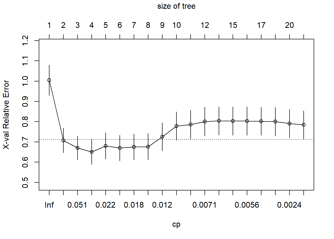

cp_table_reg <- tree_reg$cptable
best_row_reg <- which.min(cp_table_reg[, "xerror"])
best_cp_reg <- cp_table_reg[best_row_reg, "CP"]

pruned_reg <- prune(tree_reg, cp = best_cp_reg)

rpart.plot(pruned_reg, fallen.leaves = TRUE, cex = 0.75)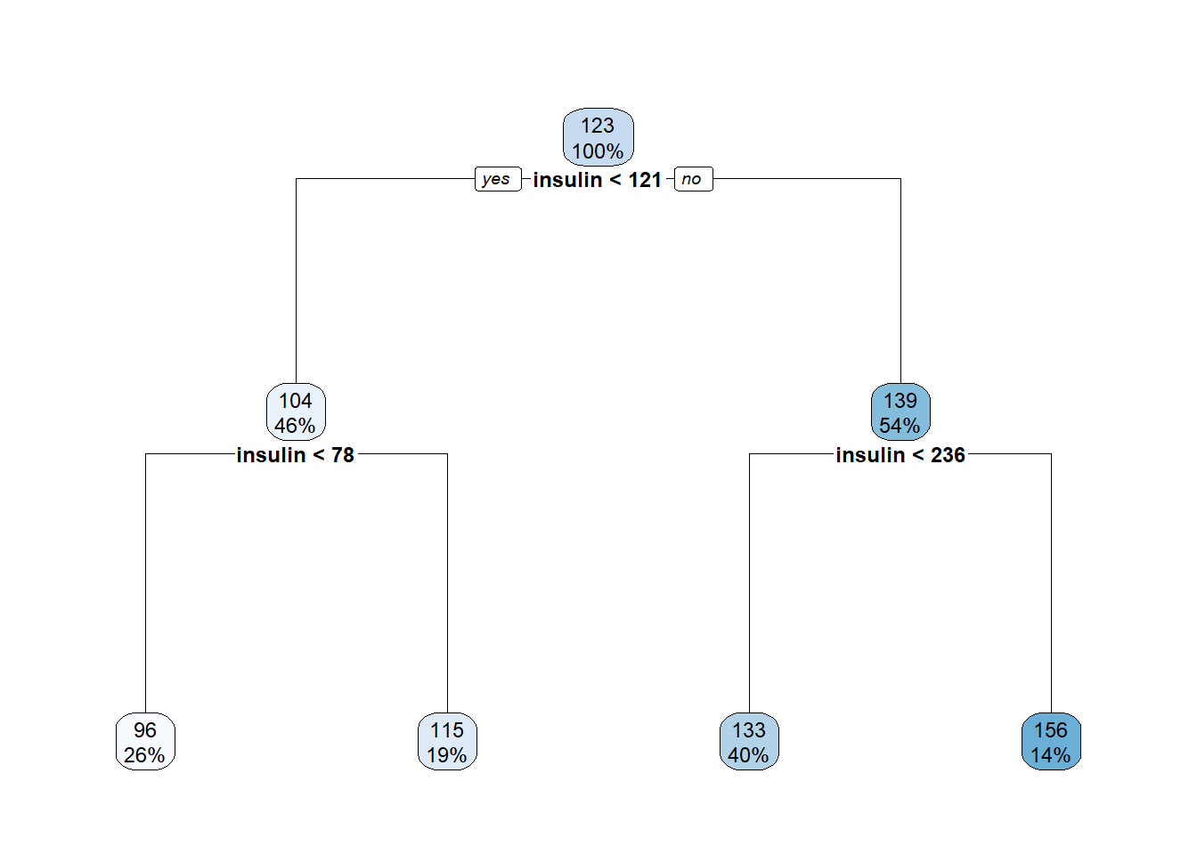

cp_table_reg <- as.data.frame(tree_reg$cptable)

root_mse <- tree_reg$frame$dev[1] / tree_reg$frame$n[1]
root_rmse <- sqrt(root_mse)

pruning_path_reg <- cp_table_reg |>
  dplyr::mutate(
    n_leaves = nsplit + 1,
    train_RMSE = sqrt(`rel error`) * root_rmse,
    cv_RMSE = sqrt(xerror) * root_rmse,
    cv_RMSE_se = sqrt(xstd) * root_rmse
  ) |>
  dplyr::select(CP, nsplit, n_leaves, train_RMSE, cv_RMSE, cv_RMSE_se)

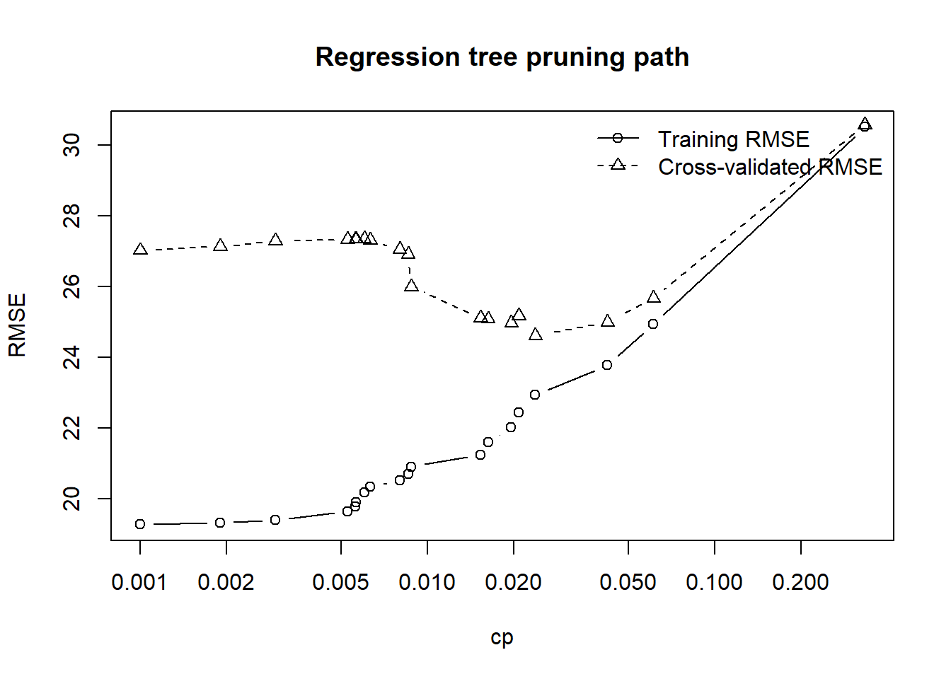
knitr::kable(pruning_path_reg, digits = 3)

CP	nsplit	n_leaves	train_RMSE	cv_RMSE	cv_RMSE_se
0.332	0	1	30.512	30.582	8.376
0.061	1	2	24.937	25.668	7.499
0.042	2	3	23.769	24.989	7.395
0.024	3	4	22.927	24.612	7.552
0.021	4	5	22.440	25.166	7.751
0.020	5	6	22.006	24.974	7.684
0.016	6	7	21.588	25.079	7.679
0.015	7	8	21.235	25.106	7.733
0.009	8	9	20.897	25.993	8.019
0.009	9	10	20.700	26.919	8.079
0.008	10	11	20.507	27.055	8.134
0.006	11	12	20.325	27.305	8.163
0.006	12	13	20.179	27.357	8.063
0.006	14	15	19.899	27.340	8.059
0.006	15	16	19.767	27.342	8.061
0.005	16	17	19.634	27.331	8.062
0.003	18	19	19.383	27.291	8.125
0.002	19	20	19.312	27.125	8.074
0.001	20	21	19.266	27.020	8.046

plot(
  pruning_path_reg$CP,
  pruning_path_reg$train_RMSE,
  type = "b",
  log = "x",
  xlab = "cp",
  ylab = "RMSE",
  main = "Regression tree pruning path"
)

lines(
  pruning_path_reg$CP,
  pruning_path_reg$cv_RMSE,
  type = "b",
  lty = 2, 
  pch=2
)

legend(
  "topright",
  legend = c("Training RMSE", "Cross-validated RMSE"),
  lty = c(1, 2),
  pch = c(1,2),
  bty = "n"
)

pred_test_reg_pruned <- predict(pruned_reg, test_reg)

rmse_test_pruned <- sqrt(mean((test_reg$glucose - pred_test_reg_pruned)^2))

comparison_reg <- data.frame(
  model = c("unpruned", "pruned"),
  test_RMSE = c(rmse_test, rmse_test_pruned),
  terminal_nodes = c(
    sum(tree_reg$frame$var == "<leaf>"),
    sum(pruned_reg$frame$var == "<leaf>")
  )
)

knitr::kable(comparison_reg, digits = 3)

model	test_RMSE	terminal_nodes
unpruned	28.551	21
pruned	25.465	4

Questions

Write your answers here or, if available, in the online form provided for the exercise.

Part 6. Final synthesis

Answer the following questions without running more code.

Questions

1. Summarize, in 5-6 lines, the full workflow followed in this lab: data preparation, train/test split, model fitting, prediction error estimation, pruning and final interpretation.

Write your answers here.

Optional extension for another dataset

If another dataset is used instead of Pima, the core workflow remains the same:

1. define the response variable;
2. identify whether the task is classification or regression;
3. split the data into training and test sets;
4. fit an initial tree;
5. interpret the main splits and terminal nodes;
6. estimate test error using an appropriate metric;
7. use cross-validation to choose the degree of pruning;
8. compare the original and pruned trees;
9. justify the final model in terms of prediction and interpretability.