Tree based methods
Alex Sanchez, Ferran Reverter and Esteban Vegas
Genetics Microbiology and Statistics Department. University of Barcelona
Introduction to Decision Trees
Motivation
- In many real-world applications, decisions need to be made based on complex, multi-dimensional data.
- One goal of statistical analysis is to provide insights and guidance to support these decisions.
- Decision trees provide a way to organize and summarize information in a way that is easy to understand and use in decision-making.
Examples
A bank needs to have a way to decide if/when a customer can be granted a loan.
A doctor may need to decide if a patient has to undergo a surgery or a less aggressive treatment.
A company may need to decide about investing in new technologies or stay with the traditional ones.
In all those cases a decision tree may provide:
- A structured approach to decision-making,
- Based on data
- That can be be easily explained and justified.
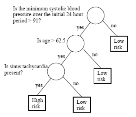
An intuitive approach
Decisions are often based on asking a sequence of yes/no questions -from more general to more specific- based on available information, whose answers induce binary splits on data that end up with some grouping or classification.
This process can be more generically stated in the context of supervised learning.
The Prediction Problem.
Let \((X, Y)\) be a r.v. with support \(\mathcal{X} \times \mathcal{Y} \subseteq \mathbb{R}^{p} \times \mathbb{R}\).
General supervised learning or prediction problem:
Training sample: \(S=\left\{\left(\boldsymbol{x}_{1}, y_{1}\right), \ldots,\left(\boldsymbol{x}_{n}, y_{n}\right)\right\}\), i.i.d. from \((\boldsymbol{X}, Y)\).
The goal is to define a function (possibly depending on the sample) \(h_{S}: \mathcal{X} \mapsto \mathcal{Y}\) such that for a new independent observation \((\boldsymbol{x}_{n+1}, y_{n+1})\) , from which we only know \(\boldsymbol{x}_{n+1}\), it happens that: \[ \hat{y}_{n+1}=h_{S}\left(x_{n+1}\right) \text { is close to } y_{n+1} \text { (in some sense). } \]
Function \(h_{S}\) is generically called a prediction function, or depending on the case, classification or regression function.
Classification and Regression
The prediction function \(h_{S}\) is said to describe a classification or a regression problem depending on the case.
If \(\mathcal{Y} \subseteq \mathbb{R}\) (or \(\mathcal{Y}\) an interval) we have a standard regression problem.
- Example: Relating Salary and demographic variables
If \(\mathcal{Y}=\{0,1\}\) (or, also, \(\mathcal{Y}=\{-1,1\}\) ) we have a problem of binary classification or discrimination.
- Example: Predicting if a “cured” disease will recidive (re-appear)
If \(\mathcal{Y}=\{1, \ldots, K\}\) (or \(\left.\mathcal{Y}=\left\{\boldsymbol{y} \in\{0,1\}^{K}: \sum_{k=1}^{K} y_{k}=1\right\}\right)\) we face a of \(K\) classes classification problem.
- Example: Classifying a tumor into one of many types
Supervised learning (1)
Probabilistic model for supervised learning
Response variable \(Y\).
Explanatory variables (features) \(\boldsymbol{X}=\left(X_{1}, \ldots, X_{p}\right)\).
Data \(\left(\boldsymbol{x}_{i}=\left(x_{i 1}, \ldots, x_{i p}\right), y_{i}\right), i=1, \ldots, n\) i.i.d. from the random variable \[ \left(\boldsymbol{X}=\left(X_{1}, \ldots, X_{p}\right), Y\right) \sim \operatorname{Pr}(\boldsymbol{X}, Y) \]
\(\operatorname{Pr}(\boldsymbol{X}, \boldsymbol{Y})\) denotes the joint distribution of \(\boldsymbol{X}\) and \(Y\).
- Main interest is predicting \(Y\) from \(\boldsymbol{X}\).
Supervised learning (2)
Given the probabilistic model it can be re-stated as learning the conditional distribution \(\operatorname{Pr}(Y \mid \boldsymbol{X})\).
In practice we focus on learning a conditional location parameter: \[ \mu(\boldsymbol{x})=\underset{\mu}{\operatorname{argmin}} \mathbb{E}(L(Y, \mu) \mid \boldsymbol{X}=\boldsymbol{x}), \] where \(L(y, \hat{y})\), loss function, measures the error of predicting \(y\) with \(\hat{y}\).
For quadratic loss, \(L(y, \hat{y})=(y-\hat{y})^{2}, \mu(x)\) is the regression function: \[ \mu(\boldsymbol{x})=\mathbb{E}(Y \mid \boldsymbol{X}=\boldsymbol{x}) \]
Introducing decision trees
A decision tree is a graphical representation of a series of decisions and their potential outcomes.
It is obtained by recursively stratifying or segmenting the feature space into a number of simple regions.
Each region (decision) corresponds to a node in the tree, and each potential outcome to a branch.
The tree structure can be used to guide decision-making based on data.
Types of decision trees
Decision trees are simple yet reliable predictors that can be use for both classification or prediction
Classification Trees are classifiers, used when the response variable is categorical
Regression Trees, are regression models used to predict the values of a numerical response variable.
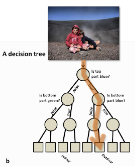
Trees vs Decision Trees
- A tree is a set of nodes and edges organized in a hierarchical fashion.
In contrast to a graph, in a tree there are no loops.
- A decision tree is a tree where each split node stores a boolean test function to be applied to the incoming data.
Each leaf stores the final answer (predictor)
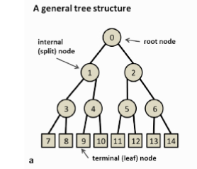
Notation used in trees (1)
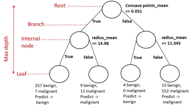
Notation used in trees (2)
A node is denoted by \(t\).
The left and right child nodes are denoted by \(t_{L}\) and \(t_{R}\)
The collection of all nodes in the tree is denoted \(T\)
The collection of all the leaf nodes is denoted \(\tilde{T}\)
A split will be denoted by \(s\).
The set of all splits is denoted by \(S\).
Tree-based models in practice
| Package | Language | Role | Notes |
|---|---|---|---|
rpart |
R | CART implementation | Standard tree fitting |
tree |
R | CART (simplified) | Mainly for teaching |
caret |
R | Modeling framework | Unified interface |
scikit-learn |
Python | CART-like trees | Standard in Python ecosystem |
- Most implementations are based on CART
- Focus on model fitting and prediction
- Details of construction will be studied next
Building Classification Trees
Building the trees
As with any model, we aim not only at construting trees.
We wish to build good trees and, if possible, optimal trees in some sense we decide.
In order to build good trees we must decide
How to construct a tree?
How to optimize the tree?
How to evaluate it?
Building a tree
A binary decision tree is built by defining a series of (recursive) splits on the feature space.
The splits are decided in such a way that the associated learning task is attained
- by setting thresholds on the variables values,
- that induce paths in the tree,
The ultimate goal of the tree is to be able to use a combination of the splits to accomplish the learning task with as small an error as possible.
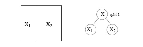
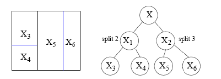
Trees partition the space
A tree represents a recursive splitting of the space.
- Every node of interest corresponds to one region in the original space.
- Two child nodes occupy two different regions.
- Together, they yield same region as that of the parent node.
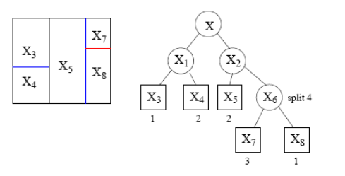
In the end, every leaf node is assigned with a class (or value) and a test point is assigned with the class (or value) of the leaf node it lands in.
The tree represents the splitting
Different splits are possible
- It is always possible to split a space in distinct ways
Some ways perform better than other for a given task, but rarely will they be perfect.
So we aim at combining splits to find a better rule.
Building a decision tree
Tree building involves the following three elements:
- The selection of the splits, i.e., how do we decide which node (region) to split and how to split it?
- How to select from the pool of candidate splits?
- What are appropriate goodness of split criteria?
- When to declare a node terminal and stop splitting?
How to assign each terminal node to a class
How to ensure the tree is the best possible we can build.
Tree construction algorithm (CART)
The most popular algorithm for buildiong trees is CART which can be schemeatically described as follows:
Initialize: all data in root node
Repeat for each node, until stopping criterion is met
2.1 Generate candidate splits
2.2 Select best split (maximize impurity reduction)
2.3 Split node into two children
CART is a greedy recursive partitioning algorithm.
TB 1.1 - Split selection
To build a Tree, questions have to be generated that induce splits based on the value of a single variable.
Ordered variable \(X_j\):
- Is \(X_j \leq c\)? for all possible thresholds \(c\).
- Split lines: parallel to the coordinates.
Categorical variables, \(X_j \in \{1, 2, \ldots, M\}\):
- Is \(X_j \in A\)?, where \(A \subseteq M\) .
The pool of candidate splits for all \(p\) variables is formed by combining all the generated questions.
With the pool of candidate splits, next step is to decide which one to use when constructing the decision tree.
TB 1.2.1 - Goodness of Split
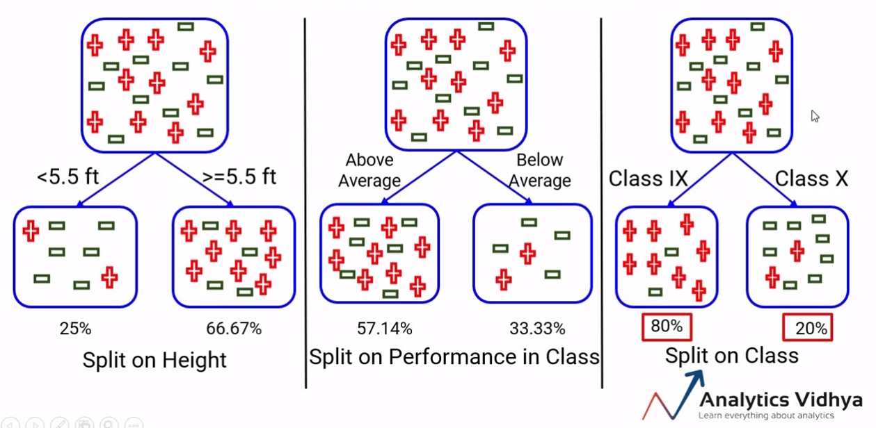
Intuitively, when we split the points we want the region corresponding to each leaf node to be “pure”.
That is, we aim at regions where most points belong to the same class.
With this goal in mind we select splits by measuring their “goodness of split” using some of the available Impurity fuctions introduced later.
TB 1.2.2 - Measuring homogeneity
In order to measure homogeneity,or as called here, purity, of splits we rely on different Impurity functions
These functions allow us to quantify the extent of homogeneity for a region containing data points from possibly different classes.
A region will be more pure or more homogeneous the less variable is the set of points it contains.
In the next image regions on the right of the image are homogeneous that is purer than the heterogeneous regions on the left.
TB 1.2.3 - Good splits vs bad splits
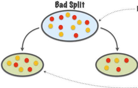
Purity not increased
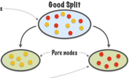
Purity increased
TB 1.2.4 - Impurity functions
An impurity function is a function \(\Phi\) defined on the set of all \(K\)-tuples of numbers \(\mathbf{p}= \left(p_{1}, \cdots, p_{K}\right)\) s.t. \(p_{j} \geq 0, \, \sum_{j=1}^K p_{j}=1\), \[ \Phi: \left(p_{1}, \cdots, p_{K}\right) \rightarrow [0,1] \]
with the properties:
- \(\Phi\) is maximum only for the uniform distribution, that is all the \(p_{j}\) are equal.
- \(\Phi\) is minimum only at points \((1,0, \ldots, 0)\),\((0,1,0, \ldots, 0)\), \(\ldots,(0,0, \ldots, 0,1)\), i.e., when the probability of being in a certain class is 1 and 0 for all the other classes.
- \(\Phi\) is a symmetric function of \(p_{1}, \cdots, p_{K}\), i.e., if we permute \(p_{j}\), \(\Phi\) remains constant.
TB 1.2.5 - Some Impurity Functions
The functions below are commonly used to measure impurity.
Entropy: \(\Phi_E (\mathbf{p}) = -\sum_{j=1}^K p_j\log (p_j)\) .
Gini Index: \(\Phi_G (\mathbf{p}) = 1-\sum_{j=1}^K p_j^2\).
Misclassification rate: \(\Phi_M (\mathbf{p}) = \sum_{i=1}^K p_j(1-p_j)\).
- In practice, only the first two are recommended because misclassification rate is not sensitive enough to differences in class probabilies.
TB 1.2.5 Impurity functions behavior
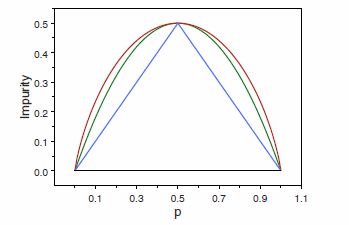
- Red curve: Entropy function (rescaled),
- Green curve: Gini index
- Blue curve: Resubstitution estimate of the misclassification rate.
TB 1.2.6 - Impurity measure of a split
- Given an impurity function \(\Phi\), a node \(t\), and given \(p(j \mid t)\), the estimated posterior probability of class \(j\) given node \(t\), the impurity measure of \(t\), \(i(t)\), is:
\[ i(t)=\phi\left (p(1 \mid t), p(2 \mid t), \ldots, p(K \mid t)\right) \]
- That is, the impurity measure of a split (or a node) is the impurity function computed on probabilities associated (conditional) with a node.
TB 1.2.7 - Goodness of a split
- Once we have defined \(i(t)\), we define the goodness of split \(s\) for node \(t\), denoted by \(\Phi(s, t)\) :
\[ \Phi(s, t)=\Delta i(s, t)=i(t)-p_{R} i\left(t_{R}\right)-p_{L} i\left(t_{L}\right) \]
The best split for the single variable \(X_{j}\) is the one that has the largest value of \(\Phi(s, t)\) over all \(s \in \mathcal{S}_{j}\), the set of possible distinct splits for \(X_{j}\).
We choose the split that maximizes impurity reduction, by using a greedy strategy: the best split is chosen locally at each step.
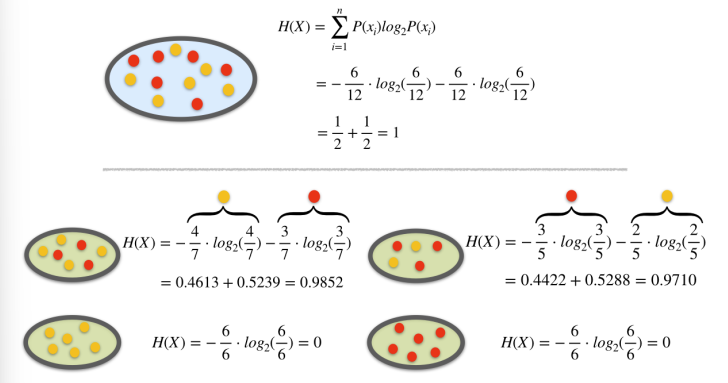
TB 1.2.8 - Entropy as an impurity measure
- The entropy of a node, \(t\), that is split in \(n\) child nodes \(t_1\), \(t_2\), …, \(t_n\), is:
\[ \Phi_E (\mathbf{p}) = H(\mathbf{t})=-\sum_{i=1}^{n} \underbrace{P\left(t_{i}\right)}_{p_i} \log _{2} P\left(t_{i}\right) \]
From here, an information gain (that is impurity decrease) measure can be introduced by comparing:
the entropy of the parent node before the split to
that of a weighted sum of the child nodes after the split where, - weights are proportional to the number of observations in each node.
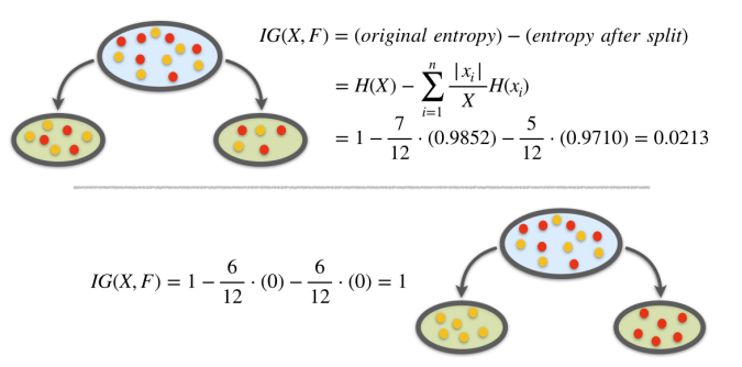
TB 1.2.9 - Information gain
- For a split \(s\) and a set of observations (a node) \(t\), information gain is defined as:
\[ \begin{aligned} & IG(t, s)=\text { (original entr.) }-(\text { entr. after split) } \\ & IG(t, s)=H(t)-\sum_{i=1}^{n} \frac{\left|t_{i}\right|}{t} H\left(x_{i}\right) \end{aligned} \]
Example 1: Pears vs Apples
Consider the problem of designing an algorithm to automatically differentiate between apples and pears (class labels) given only their width and height measurements (features).
| Width | Height | Fruit |
|---|---|---|
| 7.1 | 7.3 | Apple |
| 7.9 | 7.5 | Apple |
| 7.4 | 7.0 | Apple |
| 8.2 | 7.3 | Apple |
| 7.6 | 6.9 | Apple |
| 7.8 | 8.0 | Apple |
| 7.0 | 7.5 | Pear |
| 7.1 | 7.9 | Pear |
| 6.8 | 8.0 | Pear |
| 6.6 | 7.7 | Pear |
| 7.3 | 8.2 | Pear |
| 7.2 | 7.9 | Pear |
Example 1. Entropy Calculation
Example 1. Information Gain
TB. 1.3 Overfitting in trees
As trees grow deeper:
- They fit the training data increasingly well and
- Regions become smaller and more specific
However, small regions may contain few observations causing predictions to become unstable and sensitive to noise
This results in_
- Low training error
- Poor generalization to new data
Altogether yields an idea: It is probably better to not let the tree grow as much as it can but control its size.
TB. 1.3.1 - When to stop growing
Maximizing information gain is one possible criteria to choose among splits.
In order to avoid excessive complexity it is usually decided to stop splitting when information gain does not compensate for increase in complexity.
TB 1.3.2 Stop splitting criteria
- In practice, stop splitting is decided when: \[
\max _{s \in S} \Delta I(s, t)<\beta,
\]where:
- \(\Delta I\) represents the information gain associated with an optimal split \(s\) and a node \(t\),
- and \(\beta\) is a pre-determined threshold.
TB 1. Summary
Decision trees are built by iteratively partitioning data into smaller regions based on feature values.
Splits are aimed at producing purer nodes, that contains mostly data from one class.
Homogeneity is measured by impurity functions such as Entropy, Gini Index or Misclassification rate
The best split is chosen from candidate splits as the one that maximizes impurity reduction for example through Information Gain
Tree growth continues until impurity reduction is minimal, or a predefined depth or node size threshold is reached.
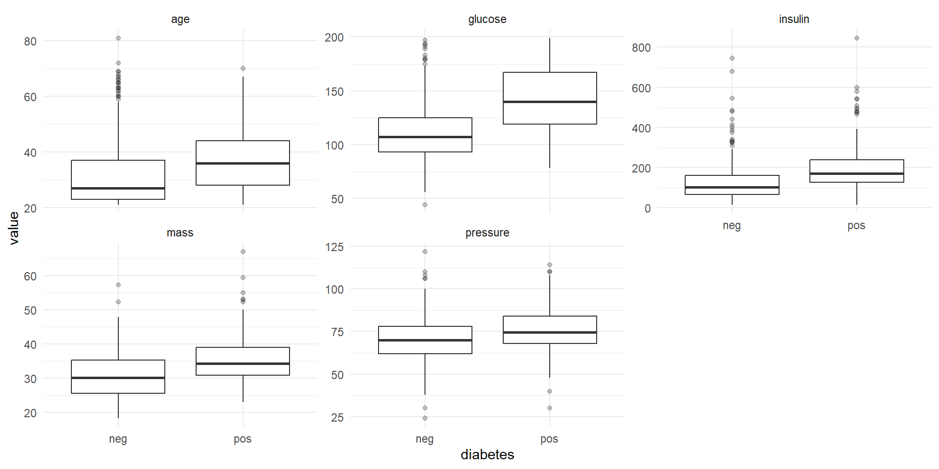
Example 2. The PIMA database
- The Pima Indian Diabetes dataset contains 768 individuals (female) and 9 clinical variables.
Rows: 768
Columns: 9
$ pregnant <dbl> 6, 1, 8, 1, 0, 5, 3, 10, 2, 8, 4, 10, 10, 1, 5, 7, 0, 7, 1, 1…
$ glucose  <dbl> 148, 85, 183, 89, 137, 116, 78, 115, 197, 125, 110, 168, 139,…
$ pressure <dbl> 72, 66, 64, 66, 40, 74, 50, NA, 70, 96, 92, 74, 80, 60, 72, N…
$ triceps  <dbl> 35, 29, NA, 23, 35, NA, 32, NA, 45, NA, NA, NA, NA, 23, 19, N…
$ insulin  <dbl> NA, NA, NA, 94, 168, NA, 88, NA, 543, NA, NA, NA, NA, 846, 17…
$ mass     <dbl> 33.6, 26.6, 23.3, 28.1, 43.1, 25.6, 31.0, 35.3, 30.5, NA, 37.…
$ pedigree <dbl> 0.627, 0.351, 0.672, 0.167, 2.288, 0.201, 0.248, 0.134, 0.158…
$ age      <dbl> 50, 31, 32, 21, 33, 30, 26, 29, 53, 54, 30, 34, 57, 59, 51, 3…
$ diabetes <fct> pos, neg, pos, neg, pos, neg, pos, neg, pos, pos, neg, pos, n…
Why these variables? (medical interlude 1)
Diabetes is a metabolic disorder related to:
- Blood sugar regulation
- Insulin function
- Long-term physiological changes
Some variables are known to be associated with diabetes risk:
- Glucose (blood sugar levels)
- Insulin (hormone regulating glucose)
- Body mass (obesity)
- Age (risk increases over time)
These variables provide indirect evidence of metabolic health
Interpreting key predictors
Glucose: High values indicate impaired blood sugar control
Insulin: Abnormal levels may reflect sugar is not being controlled (Insuline Resistance).
BMI (mass): Obesity is a major risk factor for diabetes
Age: Risk increases with cumulative metabolic stress
Blood pressure: Often associated with metabolic syndrome
The model combines these signals to predict diabetes risk
Example 2. Looking at the data
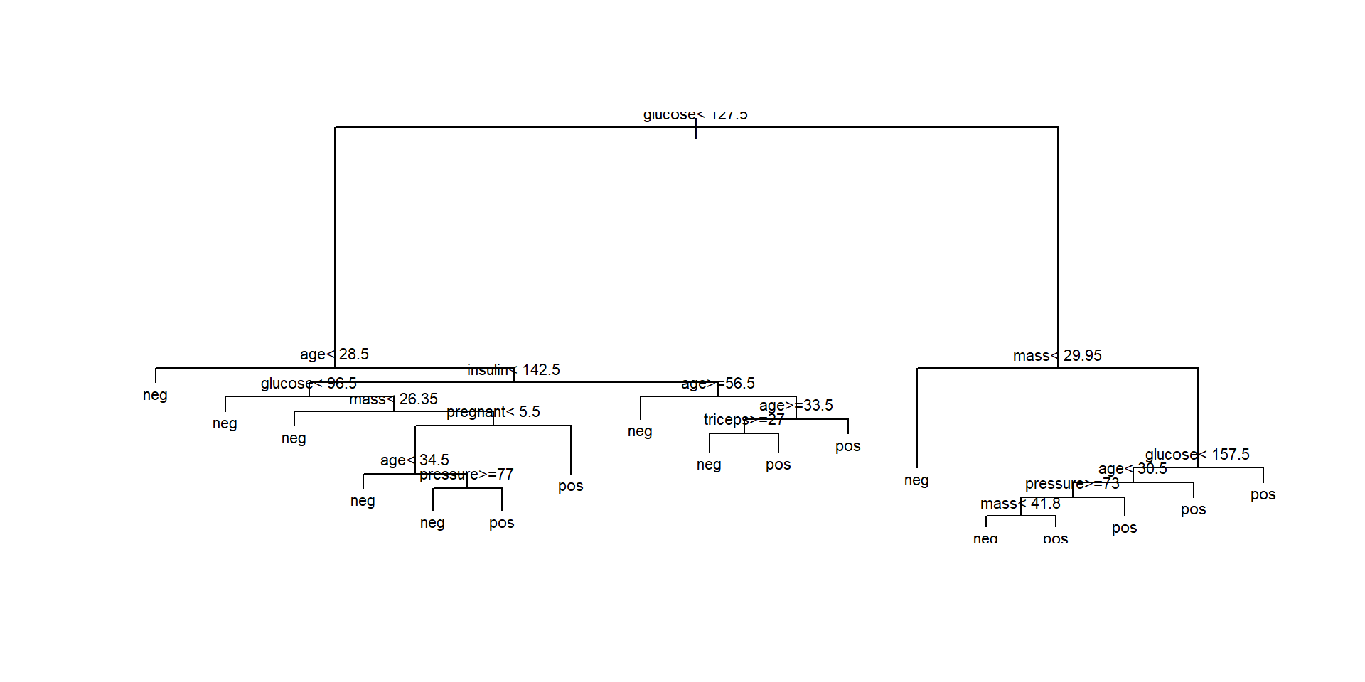
Ex. 2. Building a classification tree
We wish to predict the probability of individuals in being diabete-positive or negative.
- We start building a tree with all the variables
Ex.2. Plotting the tree (1)
Ex. 2. Plotting the tree (Nicer)
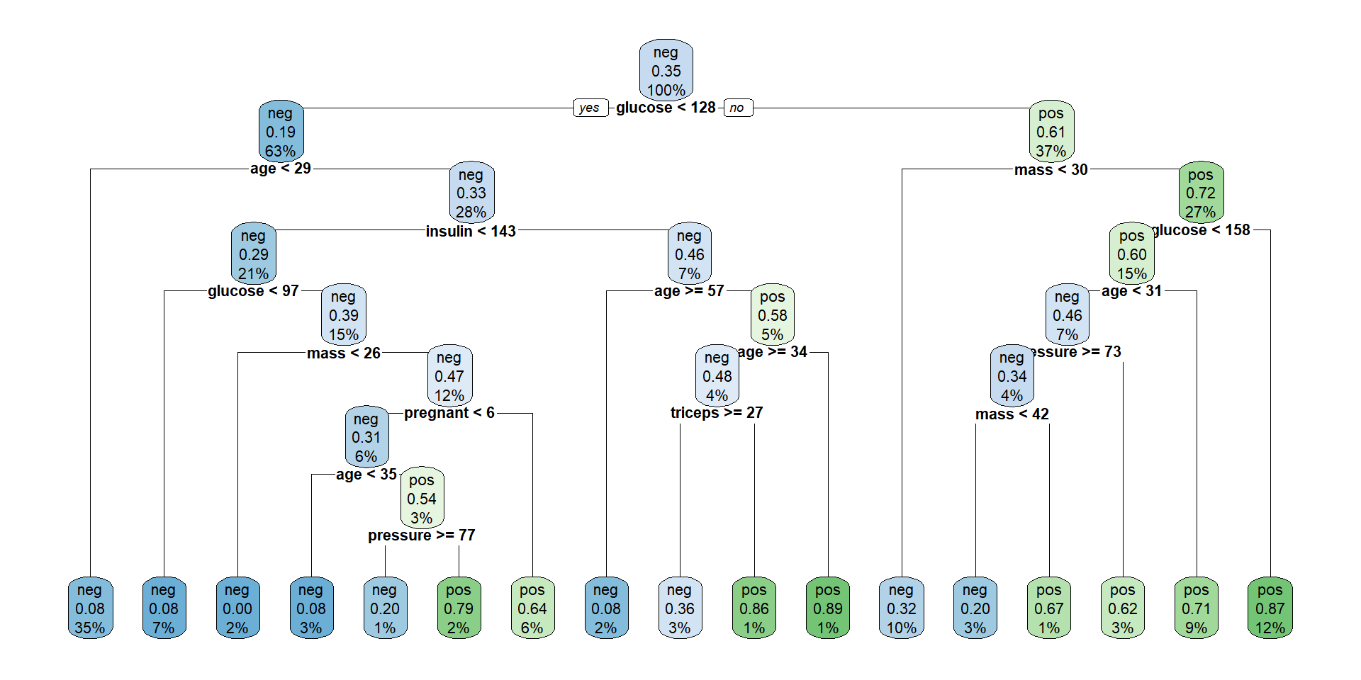
The tree plotted with the rpart.plot package.
Each node shows: (1) the predicted class (‘neg’ or ‘pos’), (2) the predicted probability, (3) the percentage of observations in the node.
Prediction with Trees
TB 2 - Class Assignment
A decision tree classifies new data points as follows.
We let a data point pass down the tree and see which leaf node it lands in.
Each leaf node defines a region where all observations share the same class.
The class of the leaf node is assigned to the new data point: all the points that land in the same leaf node will be given the same class.
Trees produce piecewise constant predictions.
TB 2.1 - Class Assignment Rules
A class assignment rule assigns a class \(j=1, \cdots, K\) to every terminal (leaf) node \(t \in \tilde{T}\).
The class assigned to node \(t\) is denoted by \(\kappa(t)\),
- E.g., if \(\kappa(t)=2\), all points in node \(t\) aree assigned to class 2.
Within each node, we estimate class probabilities from the data.
If we use 0-1 loss, the class assignment rule picks the class with maximum posterior probability: \[ \kappa(t)=\arg \max _{j} p(j \mid t) \]
This rule corresponds to minimizing the 0–1 loss within each node.
TB 2.2. Estimating the error rate (1)
Let’s assume we have built a tree and have the classes assigned for the leaf nodes.
Goal: estimate the classification error rate for this tree.
We use the resubstitution estimate \(r(t)\) for the probability of misclassification, given that a case falls into node \(t\). This is:
\[ r(t)=1-\max _{j} p(j \mid t)=1-p(\kappa(t) \mid t) \]
TB 2.3. Estimating the error rate (2)
Denote \(R(t)=r(t) p(t)\), that is the miscclassification error rate weighted by the probability of the node.
The resubstitution estimation for the overall misclassification rate \(R(T)\) of the tree classifier \(T\) is: \[ R(T)=\sum_{t \in \tilde{T}} R(t) \]
Notice that this estimate is based on training data and may underestimate the true error!
Example 2: Individual prediction
Consider individuals 521 and 562
    pregnant glucose pressure triceps insulin mass pedigree age diabetes
521        2      68       70      32      66 25.0    0.187  25      neg
562        0     198       66      32     274 41.3    0.502  28      pos
521 562
neg pos
Levels: neg posIf we follow individuals 521 and 562 along the tree, we reach the same prediction.
The tree provides not only a classification but also an explanation.
Example 2: How accurate is the model?
- It is straightforward to obtain a simple performance measure.
Example 2: Is the Tree optimal?
The question becomes harder when we go back and ask if we obtained the best possible tree.
In order to answer this question we must study tree construction in more detail.
Obtaining best trees
TB 3. Controlling tree growth
Trees obtained by looking for optimal splits tend to overfit:
- good for the data in the tree, but
- bad for generalization: tend to fail more in predictions.
Assuming we wish to control tree growth there are distinct possible approaches:
- Stop early (pre-pruning)
- Grow fully and prune later (post-pruning)
TB 3.1 Optimizing the Tree
Stopping early may prevent overfitting, but can miss important structure.
In order to reduce complexity and overfitting, while keeping the tree as good as possible, tree pruning may be applied.
Pruning works removing branches that are unlikely to improve the accuracy of the model on new data.
CART follows the second approach
TB 3.2 CART strategy for pruning
CART uses the followin strategy to build optimal trees
- Grow a large tree (overfit)
- Prune it using a penalty
- Select optimal tree size
This is known as Post-pruning approach.
TB 3.3 Pruning methods
There are different pruning methods, but the most common one is to use the cost-complexity pruning algorithm, also known as the weakest link pruning.
The algorithm works by adding a penalty term to the misclassification rate of the terminal nodes:
\[ R_\alpha(T) =R(T)+\alpha|T| \]
- \(\alpha\) is the hyper-parameter that controls the trade-off between tree complexity and accuracy.
TB 3.3 Cost-complexity pruning
First, grow a large tree that overfits the data
Then, generate a sequence of subtrees by pruning: for increasing values of \(\alpha\), smaller trees are obtained
Each subtree balances:
- fit to the data
- tree complexity
Finally, use cross-validation to select the optimal \(\alpha\)
\(\rightarrow\) This determines the final tree size
TB 3.4 CV to Select \(\alpha\)
Each sub-tree can by evaluated with cross-validation as follows:
- Split the data into K folds
- Compute prediction error for each \(\alpha\), on validation folds
- Average the error across folds
Select the value of \(\alpha\) with lowest validation error.
Ex. 3 Optimizing the tree (1)
        CP nsplit rel error   xerror     xstd
1 0.242537      0  1.000000 1.000000 0.049288
2 0.100746      1  0.757463 0.798507 0.046360
3 0.011816      2  0.656716 0.757463 0.045599
4 0.011194     10  0.555970 0.716418 0.044776
5 0.010000     16  0.488806 0.701493 0.044461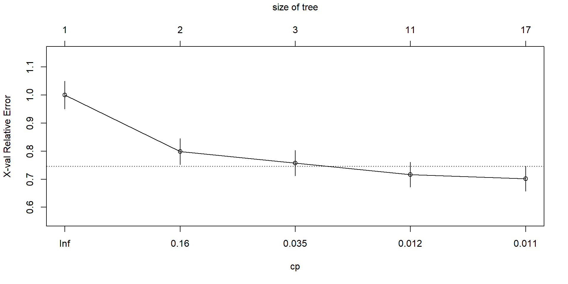
Ex 3. Building the optimal tree
[1] 0.01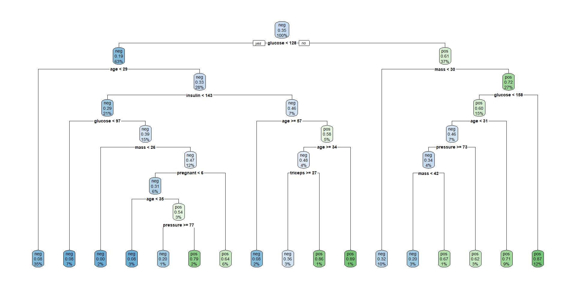
Regression Trees
Regression modelling with trees
When the response variable is numeric, decision trees are regression trees.
Option of choice for distinct reasons
- The relation between response and potential explanatory variables is not linear.
- Perform automatic variable selection.
- Easy to interpret, visualize, explain.
- Robust to outliers and can handle missing data
Classification vs Regression Trees
| Aspect | Regression Trees | Classification Trees |
|---|---|---|
| Outcome var. type | Continuous | Categorical |
| Goal | To predict a numerical value | To predict a class label |
| Splitting criteria | Mean Squared Error, Mean Abs. Error | Gini Impurity, Entropy, etc. |
| Leaf node prediction | Mean or median of the target variable in that region | Mode or majority class of the target variable … |
| Examples of use cases | Predicting housing prices, predicting stock prices | Predicting customer churn, predicting high/low risk in diease |
| Evaluation metric | Mean Squared Error, Mean Absolute Error, R-square | Accuracy, Precision, Recall, F1-score, etc. |
Regression tree example
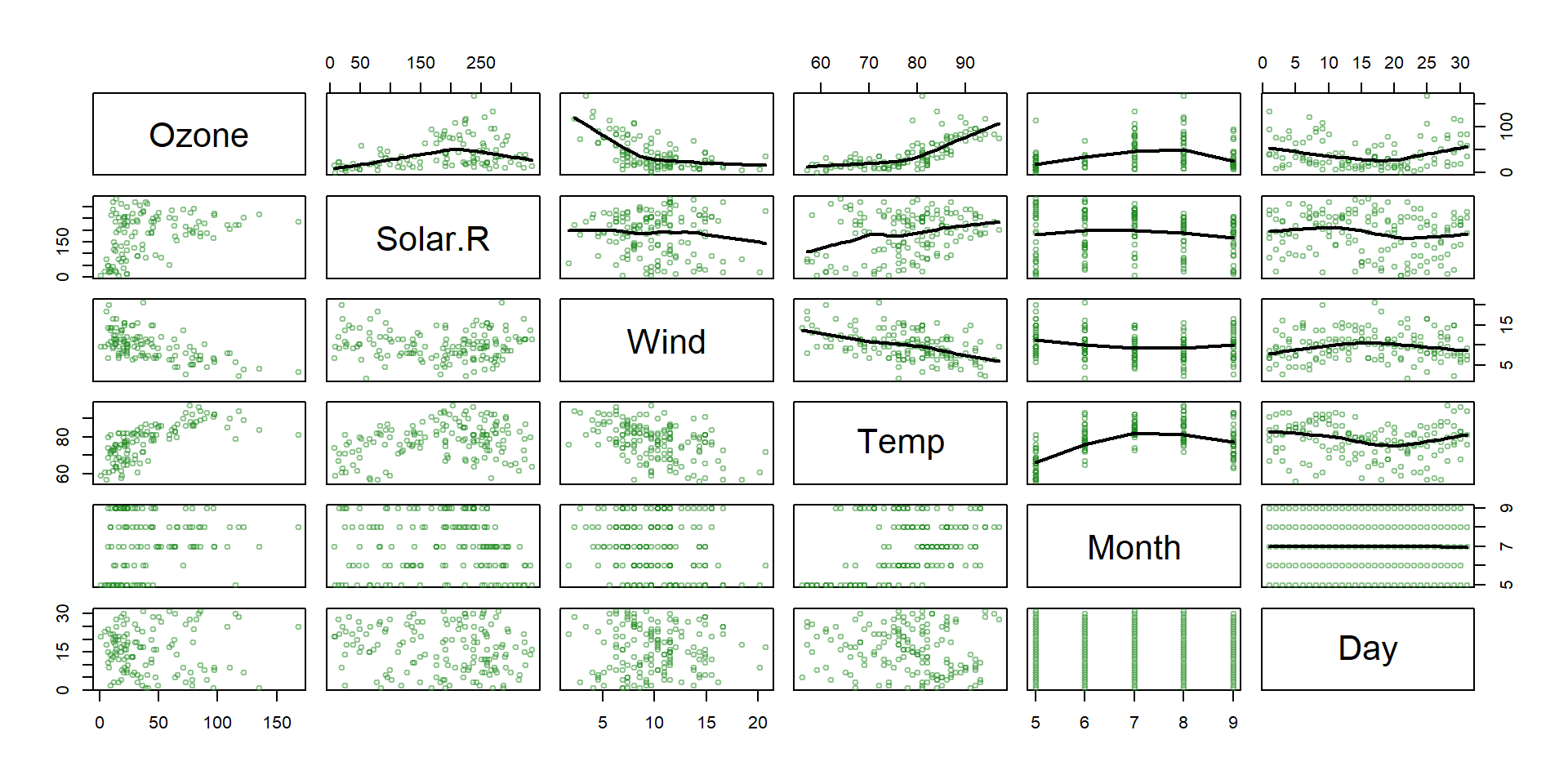
- The
airqualitydataset from thedatasetspackage contains daily air quality measurements in New York from May through September of 1973 (153 days). - The main variables include:
- Ozone: the mean ozone (in parts per billion) …
- Solar.R: the solar radiation (in Langleys) …
- Wind: the average wind speed (in mph) …
- Temp: the maximum daily temperature (ºF) …
- Main goal : Predict ozone concentration.
Non linear relationships!
Building the tree (1): Splitting
- Consider:
- all predictors \(X_1, \dots, X_n\), and
- all values of cutpoint \(s\) for each predictor and
- For each predictor find boxes \(R_1, \ldots, R_J\) that minimize the RSS, given by:
\[ \sum_{j=1}^J \sum_{i \in R_j}\left(y_i-\hat{y}_{R_j}\right)^2 \]
where \(\hat{y}_{R_j}\) is the mean response for the training observations within the \(j\) th box.
Building the tree (2): Splitting
- To do this, define the pair of half-planes
\[ R_1(j, s)=\left\{X \mid X_j<s\right\} \text { and } R_2(j, s)=\left\{X \mid X_j \geq s\right\} \]
and seek the value of \(j\) and \(s\) that minimize the equation:
\[ \sum_{i: x_i \in R_1(j, s)}\left(y_i-\hat{y}_{R_1}\right)^2+\sum_{i: x_i \in R_2(j, s)}\left(y_i-\hat{y}_{R_2}\right)^2. \]
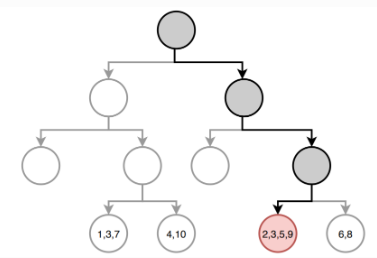
Building the tree (3): Prediction
Once the regions have been created we predict the response using the mean of the trainig observations in the region to which that observation belongs.
In the example, for an observation belonging to the shaded region, the prediction would be:
\[ \hat{y} =\frac{1}{4}(y_2+y_3+y_5+y_9) \]
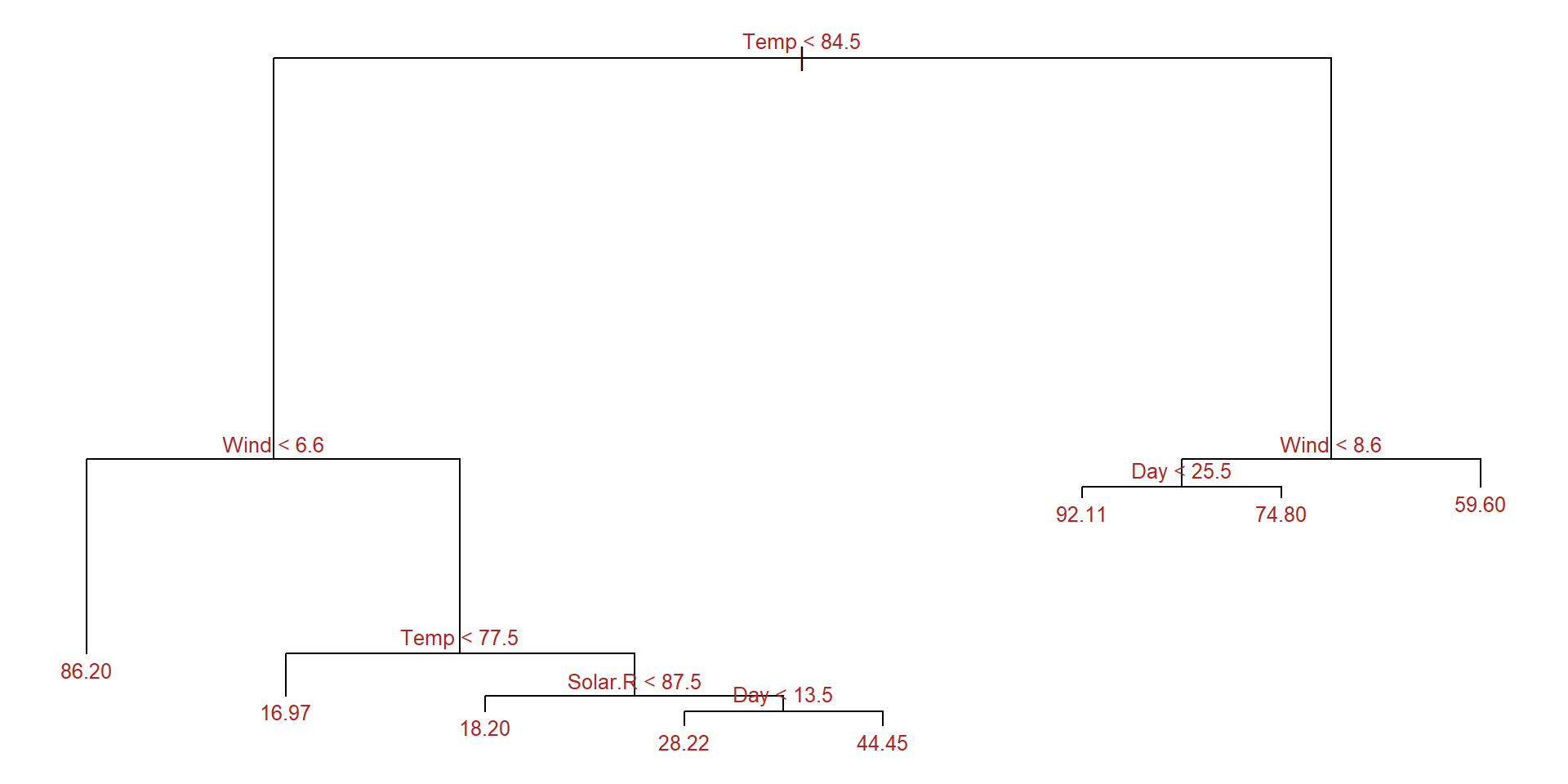
Example: A regression tree
set.seed(123)
train <- sample(1:nrow(aq), size = nrow(aq)*0.7)
aq_train <- aq[train,]
aq_test  <- aq[-train,]
aq_regresion <- tree::tree(formula = Ozone ~ .,
                           data = aq_train, split = "deviance")
summary(aq_regresion)
Regression tree:
tree::tree(formula = Ozone ~ ., data = aq_train, split = "deviance")
Variables actually used in tree construction:
[1] "Temp"    "Wind"    "Solar.R" "Day"
Number of terminal nodes:  8
Residual mean deviance:  285.6 = 21420 / 75
Distribution of residuals:
    Min.  1st Qu.   Median     Mean  3rd Qu.     Max.
-58.2000  -7.9710  -0.4545   0.0000   5.5290  81.8000
Example: Plot the tree
Error estimation and optimization for regression trees
Prunning the tree (1)
- As before, cost-complexity prunning can be applied
- We consider a sequence of trees indexed by a nonnegative tuning parameter \(\alpha\).
- For each value of \(\alpha\) there corresponds a subtree \(T \subset T_0\) such that:
\[ \sum_{m=1}^{|T|} \sum_{y_i \in R_m} \left(y_i -\hat{y}_{R_m}\right)^2+ \alpha|T|\quad (*) \label{prunning} \]
is as small as possible.
Tuning parameter \(\alpha\)
- \(\alpha\) controls a trade-off between the subtree’s complexity and its fit to the training data.
- When \(\alpha=0\), then the subtree \(T\) will simply equal \(T_0\).
- As \(\alpha\) increases, there is a price to pay for having a tree with many terminal nodes, and so (*) will tend to be minimized for a smaller subtree.
- Equation (*1) is reminiscent of the lasso.
- \(\alpha\) can be chosen by cross-validation .
Optimizing the tree (\(\alpha\))
Use recursive binary splitting to grow a large tree on the training data, stopping only when each terminal node has fewer than some minimum number of observations.
Apply cost complexity pruning to the large tree in order to obtain a sequence of best subtrees, as a function of \(\alpha\).
Use K-fold cross-validation to choose \(\alpha\). That is, divide the training observations into \(K\) folds. For each \(k=1, \ldots, K\) :
- Repeat Steps 1 and 2 on all but the \(k\) th fold of the training data.
- Evaluate the mean squared prediction error on the data in the left-out \(k\) th fold, as a function of \(\alpha\).
Average the results for each value of \(\alpha\). Pick \(\alpha\) to minimize the average error.
- Return the subtree from Step 2 that corresponds to the chosen value of \(\alpha\).
Example: Prune the tree
cv_aq <- tree::cv.tree(aq_regresion, K = 5)
optimal_size <-  rev(cv_aq$size)[which.min(rev(cv_aq$dev))]
aq_final_tree <- tree::prune.tree(
                 tree = aq_regresion,
                 best = optimal_size
               )
summary(aq_final_tree)
Regression tree:
tree::tree(formula = Ozone ~ ., data = aq_train, split = "deviance")
Variables actually used in tree construction:
[1] "Temp"    "Wind"    "Solar.R" "Day"
Number of terminal nodes:  8
Residual mean deviance:  285.6 = 21420 / 75
Distribution of residuals:
    Min.  1st Qu.   Median     Mean  3rd Qu.     Max.
-58.2000  -7.9710  -0.4545   0.0000   5.5290  81.8000
In this example pruning does not improve the tree.
Advantages and disadvantages of trees
Trees have many advantages
Trees are very easy to explain to people.
Decision trees may be seen as good mirrors of human decision-making.
Trees can be displayed graphically, and are easily interpreted even by a non-expert.
Trees can easily handle qualitative predictors without the need to create dummy variables.
But they come at a price
Trees generally do not have the same level of predictive accuracy as sorne of the other regression and classification approaches.
Additionally, trees can be very non-robust: a small change in the data can cause a large change in the final estimated tree.
References and Resources
References
Efron, B., Hastie T. (2016) Computer Age Statistical Inference. Cambridge University Press. Web site
Hastie, T., Tibshirani, R., & Friedman, J. (2009). The elements of statistical learning: Data mining, inference, and prediction. Springer.
James, G., Witten, D., Hastie, T., & Tibshirani, R. (2013). An introduction to statistical learning (Vol. 112). Springer. Web site
Complementary references
Breiman, L., Friedman, J., Stone, C. J., & Olshen, R. A. (1984). Classification and regression trees. CRC press.
Brandon M. Greenwell (202) Tree-Based Methods for Statistical Learning in R. 1st Edition. Chapman and Hall/CRC DOI: https://doi.org/10.1201/9781003089032
Genuer R., Poggi, J.M. (2020) Random Forests with R. Springer ed. (UseR!)
Resources
Applied Data Mining and Statistical Learning (Penn Statte-University)
An Introduction to Recursive Partitioning Using the RPART Routines