Machine Learning 4 Metabolomics
Decision Trees, Random Forests and SVMs
Genetics Microbiology and Statistics Department. University of Barcelona
Introduction to Decision Trees
Motivation
- In many real-world applications, decisions need to be made based on complex, multi-dimensional data.
- One goal of statistical analysis is to provide insights and guidance to support these decisions.
- Decision trees provide a way to organize and summarize information in a way that is easy to understand and use in decision-making.
Examples
A bank needs to have a way to decide if/when a customer can be granted a loan.
A doctor may need to decide if a patient has to undergo a surgery or a less aggressive treatment.
A company may need to decide about investing in new technologies or stay with the traditional ones.
In all those cases a decision tree may provide a structured approach to decision-making that is based on data and can be easily explained and justified.
An intuitive approach
Decisions are often based on asking several questions on available information whose answers induce binary splits on data that end up with some grouping or classification.
So, what is a decision tree?
A decision tree is a graphical representation of a series of decisions and their potential outcomes.
It is obtained by recursively stratifying or segmenting the feature space into a number of simple regions.
Each region (decision) corresponds to a node in the tree, and each potential outcome to a branch.
The tree structure can be used to guide decision-making based on data.
What do we need to learn?
We need context:
When is it appropriate to rely on decision trees?
When would other approaches be preferable?
What type of decision trees can be used?
We need to know how to build good trees
- How do we construct a tree?
- How do we optimize the tree?
- How do we evaluate it?
More about context
Decision trees are non parametric, data guided predictors, well suited in many situations such as:
- Non-linear relationships.
- High-dimensional data.
- Interaction between variables exist.
- Mixed data types.
They are not so appropriate for complex datasets, or complex problems, that require expert knowledge.
Types of decision trees
Classification Trees are built when the response variable is categorical.
- They aim to classify a new observation based on the values of the predictor variables.
Regression Trees are used when the response variable is numerical.
- They aim to predict the value of a continuous response variable based on the values of the predictor variables.
Tree building with R
Tree building with Python
| Package | Algorithm | Dataset size | Missing data handling | Ensemble methods | Visual repr | User interface |
|---|---|---|---|---|---|---|
scikit-learn |
CART (DecisionTreeClassifier) | Small to large | Can handle NaN | Yes | Yes (using Graphviz) | Simple |
dtreeviz |
CART (DecisionTree) | Small to large | Can handle NaN | No | Yes | Simple |
xgboost |
Gradient Boosting | Medium to large | Requires imputation | Yes | No | Complex |
lightgbm |
Gradient Boosting | Medium to large | Requires imputation | Yes | No | Complex |
Starting with an example
- The Pima Indian Diabetes dataset contains 768 individuals (female) and 9 clinical variables.
Rows: 768
Columns: 9
$ pregnant <dbl> 6, 1, 8, 1, 0, 5, 3, 10, 2, 8, 4, 10, 10, 1, 5, 7, 0, 7, 1, 1…
$ glucose  <dbl> 148, 85, 183, 89, 137, 116, 78, 115, 197, 125, 110, 168, 139,…
$ pressure <dbl> 72, 66, 64, 66, 40, 74, 50, NA, 70, 96, 92, 74, 80, 60, 72, N…
$ triceps  <dbl> 35, 29, NA, 23, 35, NA, 32, NA, 45, NA, NA, NA, NA, 23, 19, N…
$ insulin  <dbl> NA, NA, NA, 94, 168, NA, 88, NA, 543, NA, NA, NA, NA, 846, 17…
$ mass     <dbl> 33.6, 26.6, 23.3, 28.1, 43.1, 25.6, 31.0, 35.3, 30.5, NA, 37.…
$ pedigree <dbl> 0.627, 0.351, 0.672, 0.167, 2.288, 0.201, 0.248, 0.134, 0.158…
$ age      <dbl> 50, 31, 32, 21, 33, 30, 26, 29, 53, 54, 30, 34, 57, 59, 51, 3…
$ diabetes <fct> pos, neg, pos, neg, pos, neg, pos, neg, pos, pos, neg, pos, n…
Looking at the data
- These Variables are known to be related with cardiovascular diseases.
- It seems intuitive to use these variables to decide if a person is affected by diabetes
             p0      p25      p50       p75   p100  hist
diabetes     NA       NA       NA        NA     NA  <NA>
pregnant  0.000  1.00000   3.0000   6.00000  17.00 ▇▃▂▁▁
glucose  44.000 99.00000 117.0000 141.00000 199.00 ▁▇▇▃▂
pressure 24.000 64.00000  72.0000  80.00000 122.00 ▁▃▇▂▁
triceps   7.000 22.00000  29.0000  36.00000  99.00 ▆▇▁▁▁
insulin  14.000 76.25000 125.0000 190.00000 846.00 ▇▂▁▁▁
mass     18.200 27.50000  32.3000  36.60000  67.10 ▅▇▃▁▁
pedigree  0.078  0.24375   0.3725   0.62625   2.42 ▇▃▁▁▁
age      21.000 24.00000  29.0000  41.00000  81.00 ▇▃▁▁▁
Predicting Diabetes onset
We wish to predict the probability of individuals in being diabete-positive or negative.
- We start building a tree with all the variables
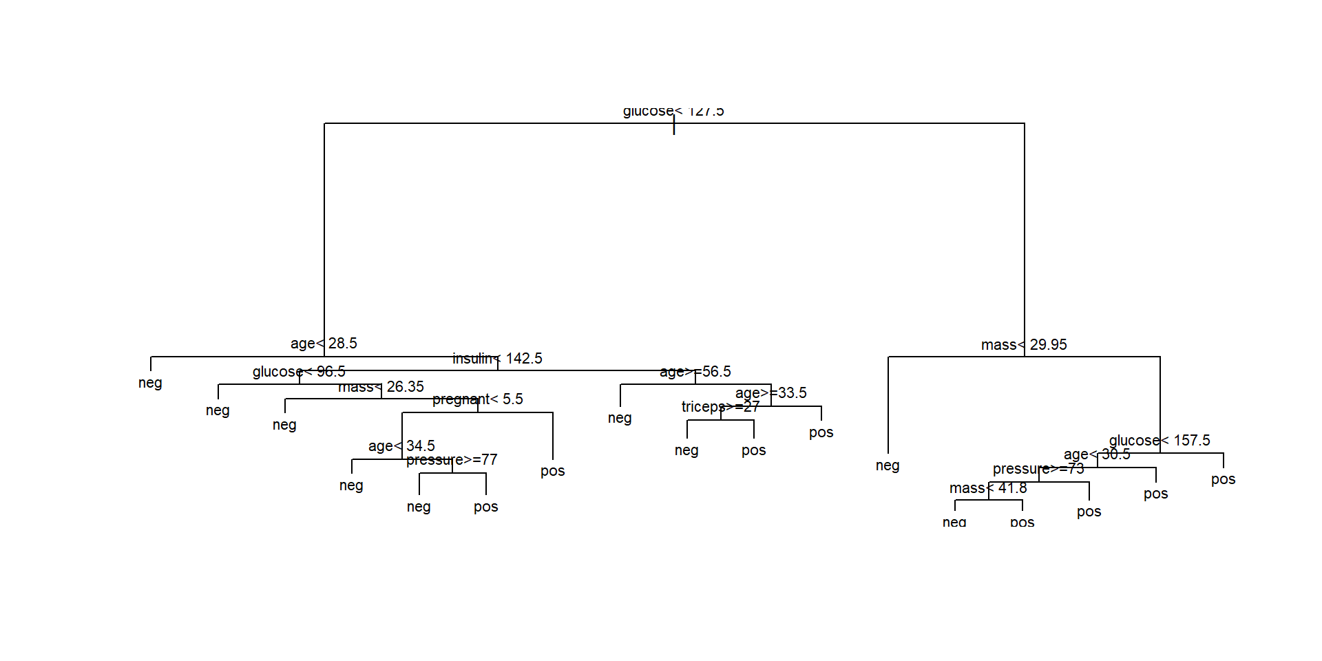
- A simple visualization illustrates how it proceeds
Viewing the tree as text
n= 768

node), split, n, loss, yval, (yprob)
      * denotes terminal node

  1) root 768 268 neg (0.65104167 0.34895833)
    2) glucose< 127.5 485  94 neg (0.80618557 0.19381443)
      4) age< 28.5 271  23 neg (0.91512915 0.08487085) *
      5) age>=28.5 214  71 neg (0.66822430 0.33177570)
       10) insulin< 142.5 164  48 neg (0.70731707 0.29268293)
         20) glucose< 96.5 51   4 neg (0.92156863 0.07843137) *
         21) glucose>=96.5 113  44 neg (0.61061947 0.38938053)
           42) mass< 26.35 19   0 neg (1.00000000 0.00000000) *
           43) mass>=26.35 94  44 neg (0.53191489 0.46808511)
             86) pregnant< 5.5 49  15 neg (0.69387755 0.30612245)
              172) age< 34.5 25   2 neg (0.92000000 0.08000000) *
              173) age>=34.5 24  11 pos (0.45833333 0.54166667)
                346) pressure>=77 10   2 neg (0.80000000 0.20000000) *
                347) pressure< 77 14   3 pos (0.21428571 0.78571429) *
             87) pregnant>=5.5 45  16 pos (0.35555556 0.64444444) *
       11) insulin>=142.5 50  23 neg (0.54000000 0.46000000)
         22) age>=56.5 12   1 neg (0.91666667 0.08333333) *
         23) age< 56.5 38  16 pos (0.42105263 0.57894737)
           46) age>=33.5 29  14 neg (0.51724138 0.48275862)
             92) triceps>=27 22   8 neg (0.63636364 0.36363636) *
             93) triceps< 27 7   1 pos (0.14285714 0.85714286) *
           47) age< 33.5 9   1 pos (0.11111111 0.88888889) *
    3) glucose>=127.5 283 109 pos (0.38515901 0.61484099)
      6) mass< 29.95 75  24 neg (0.68000000 0.32000000) *
      7) mass>=29.95 208  58 pos (0.27884615 0.72115385)
       14) glucose< 157.5 116  46 pos (0.39655172 0.60344828)
         28) age< 30.5 50  23 neg (0.54000000 0.46000000)
           56) pressure>=73 29  10 neg (0.65517241 0.34482759)
            112) mass< 41.8 20   4 neg (0.80000000 0.20000000) *
            113) mass>=41.8 9   3 pos (0.33333333 0.66666667) *
           57) pressure< 73 21   8 pos (0.38095238 0.61904762) *
         29) age>=30.5 66  19 pos (0.28787879 0.71212121) *
15) glucose>=157.5 92 12 pos (0.13043478 0.86956522) *- This representation shows the variables and split values that have been selected by the algorithm.
- It can be used to classify (new) individuals following the decisions (splits) from top to bottom.
Plotting the tree (1)
Plotting the tree (Nicer)
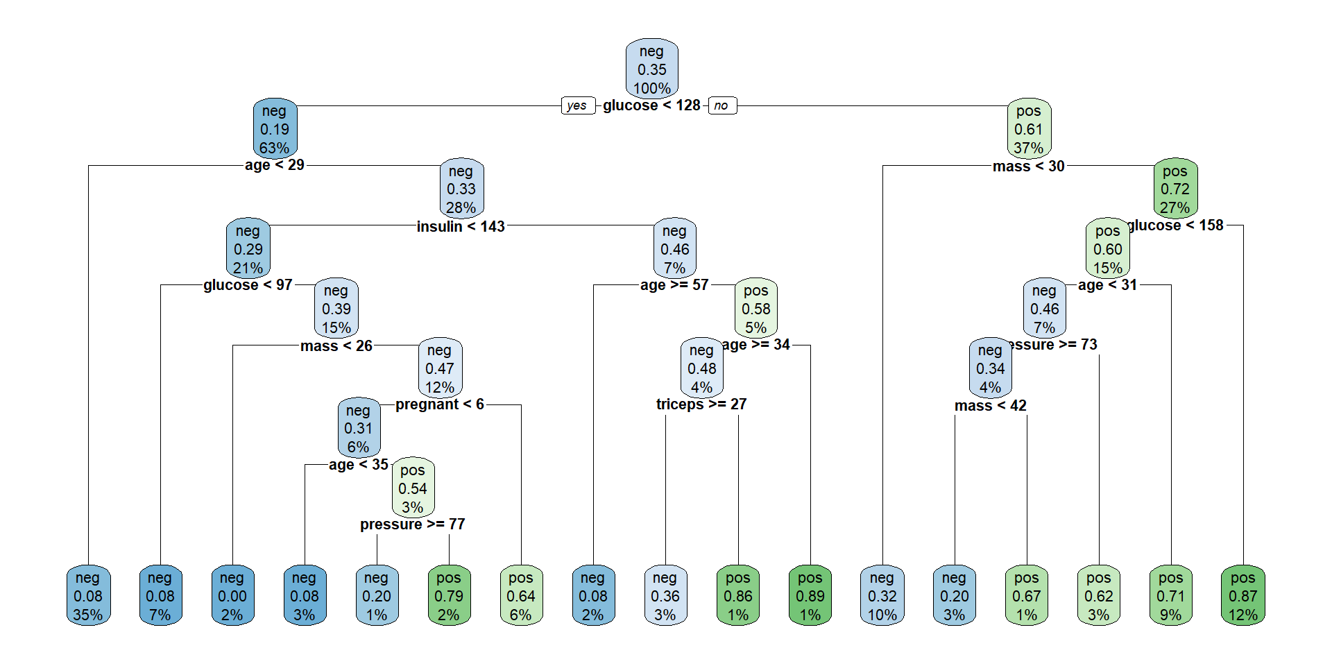
The tree plotted with the rpart.plot package.
Each node shows: (1) the predicted class (‘neg’ or ‘pos’), (2) the predicted probability, (3) the percentage of observations in the node.
Individual prediction
Consider individuals 521 and 562
    pregnant glucose pressure triceps insulin mass pedigree age diabetes
521        2      68       70      32      66 25.0    0.187  25      neg
562        0     198       66      32     274 41.3    0.502  28      pos
521 562
neg pos
Levels: neg posIf we follow individuals 521 and 562 along the tree, we reach the same prediction.
The tree provides not only a classification but also an explanation.
How accurate is the model?
- It is straightforward to obtain a simple performance measure.
predicted.classes<- predict(model1, PimaIndiansDiabetes2, "class")
mean(predicted.classes == PimaIndiansDiabetes2$diabetes)
[1] 0.8294271The question becomes harder when we go back and ask if we obtained the best possible tree.
In order to answer this question we must study tree construction in more detail.
Building the trees
As with any model, we aim not only at construting trees.
We wish to build good trees and, if possible, optimal trees in some sense we decide.
In order to build good trees we must decide
How to construct a tree?
How to optimize the tree?
How to evaluate it?
Prediction with Trees
The decision tree classifies new data points as follows.
We let a data point pass down the tree and see which leaf node it lands in.
The class of the leaf node is assigned to the new data point. Basically, all the points that land in the same leaf node will be given the same class.
This is similar to k-means or any prototype method.
Regression modelling with trees
When the response variable is numeric, decision trees are regression trees.
Option of choice for distinct reasons
- The relation between response and potential explanatory variables is not linear.
- Perform automatic variable selection.
- Easy to interpret, visualize, explain.
- Robust to outliers and can handle missing data
Classification vs Regression Trees
| Aspect | Regression Trees | Classification Trees |
|---|---|---|
| Outcome var. type | Continuous | Categorical |
| Goal | To predict a numerical value | To predict a class label |
| Splitting criteria | Mean Squared Error, Mean Abs. Error | Gini Impurity, Entropy, etc. |
| Leaf node prediction | Mean or median of the target variable in that region | Mode or majority class of the target variable ... |
| Examples of use cases | Predicting housing prices, predicting stock prices | Predicting customer churn, predicting high/low risk in diease |
| Evaluation metric | Mean Squared Error, Mean Absolute Error, R-square | Accuracy, Precision, Recall, F1-score, etc. |
Regression tree example
- The
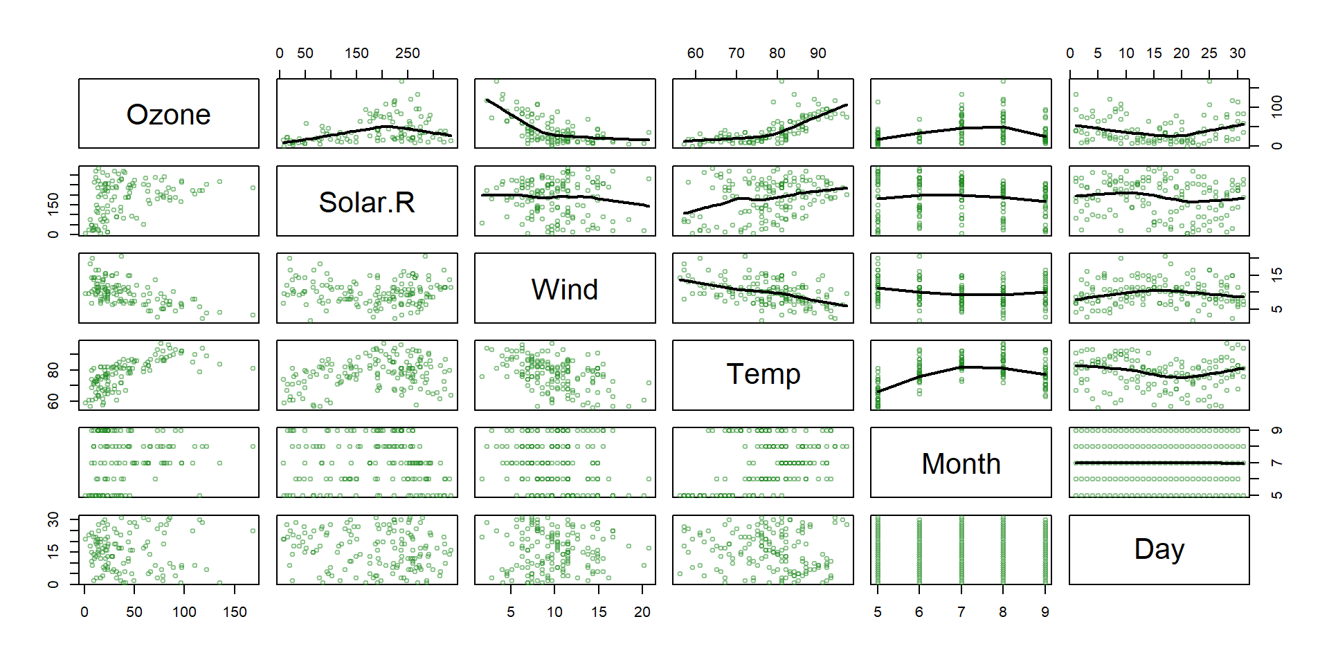
airqualitydataset from thedatasetspackage contains daily air quality measurements in New York from May through September of 1973 (153 days). - The main variables include:
- Ozone: the mean ozone (in parts per billion) …
- Solar.R: the solar radiation (in Langleys) …
- Wind: the average wind speed (in mph) …
- Temp: the maximum daily temperature (ºF) …
- Main goal : Predict ozone concentration.
Non linear relationships!
Building the tree (1): Splitting
- Consider:
- all predictors \(X_1, \dots, X_n\), and
- all values of cutpoint \(s\) for each predictor and
- For each predictor find boxes \(R_1, \ldots, R_J\) that minimize the RSS, given by:
\[ \sum_{j=1}^J \sum_{i \in R_j}\left(y_i-\hat{y}_{R_j}\right)^2 \]
where \(\hat{y}_{R_j}\) is the mean response for the training observations within the \(j\) th box.
Building the tree (2): Splitting
- To do this, define the pair of half-planes
\[ R_1(j, s)=\left\{X \mid X_j<s\right\} \text { and } R_2(j, s)=\left\{X \mid X_j \geq s\right\} \]
and seek the value of \(j\) and \(s\) that minimize the equation:
\[ \sum_{i: x_i \in R_1(j, s)}\left(y_i-\hat{y}_{R_1}\right)^2+\sum_{i: x_i \in R_2(j, s)}\left(y_i-\hat{y}_{R_2}\right)^2. \]
Building the tree (3): Prediction
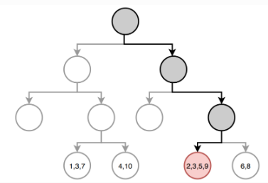
Once the regions have been created we predict the response using the mean of the trainig observations in the region to which that observation belongs.
In the example, for an observation belonging to the shaded region, the prediction would be:
\[ \hat{y} =\frac{1}{4}(y_2+y_3+y_5+y_9) \]
Example: A regression tree
set.seed(123)
train <- sample(1:nrow(aq), size = nrow(aq)*0.7)
aq_train <- aq[train,]
aq_test  <- aq[-train,]
aq_regresion <- tree::tree(formula = Ozone ~ .,
                           data = aq_train, split = "deviance")
summary(aq_regresion)
Regression tree:
tree::tree(formula = Ozone ~ ., data = aq_train, split = "deviance")
Variables actually used in tree construction:
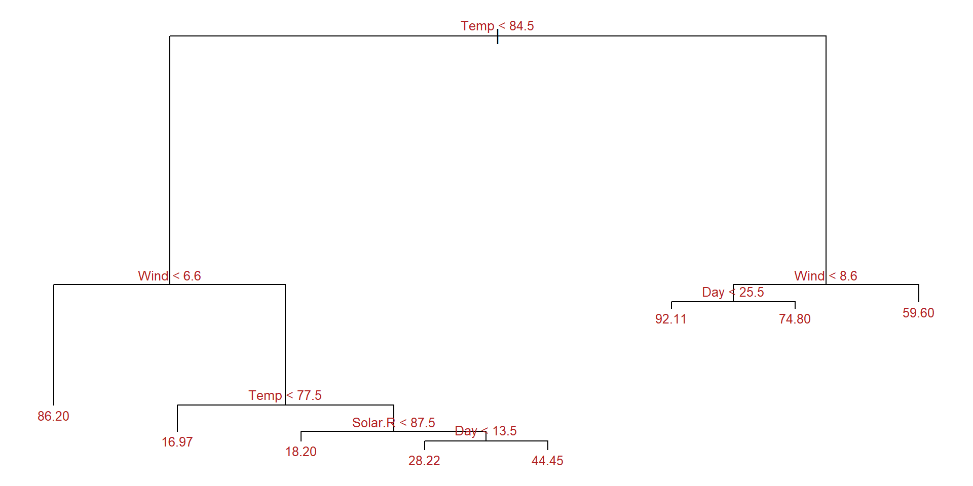
[1] "Temp"    "Wind"    "Solar.R" "Day"
Number of terminal nodes:  8
Residual mean deviance:  285.6 = 21420 / 75
Distribution of residuals:
    Min.  1st Qu.   Median     Mean  3rd Qu.     Max.
-58.2000  -7.9710  -0.4545   0.0000   5.5290  81.8000
Example: Plot the tree
Trees have many advantages
Trees are very easy to explain to people.
Decision trees may be seen as good mirrors of human decision-making.
Trees can be displayed graphically, and are easily interpreted even by a non-expert.
Trees can easily handle qualitative predictors without the need to create dummy variables.
But they come at a price
Trees generally do not have the same level of predictive accuracy as sorne of the other regression and classification approaches.
Additionally, trees can be very non-robust: a small change in the data can cause a large change in the final estimated tree.
Introduction to Ensembles
Weak learners
Models that perform only slightly better than random guessing are called weak learners (Bishop 2007).
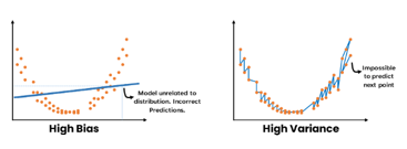
Weak learners low predictive accuracy may be due, to the predictor having high bias or high variance.
Trees may be weak learners
- May be sensitive to small changes in training data that lead to very different tree structure.
- High sensitivity implies predictions are highly variable
- They are greedy algorithms making locally optimal decisions at each node without considering the global optimal solution.
- This can lead to suboptimal splits and ultimately a weaker predictive performance.
There’s room for improvement
In many situations trees may be a good option (e.g. for simplicity and interpretability)
But there are issues that, if solved, may improve performance.
It is to be noted, too, that these problems are not unique to trees.
- Other simple models such as linear regression may be considered as weakl learners in may situations.
The bias-variance trade-off
- When we try to improve weak learners we need to deal with the bias-variance trade-off.
How to deal with such trade-off
How can a model be made less variable or less biased without this increasing its bias or variance?
There are distinct appraches to deal with this problem
- Regularization,
- Feature engineering,
- Model selection
- Ensemble learning
Ensemble learners
Ensemble learning takes a distinct based on “the wisdom of crowds”.
Predictors, also called, ensembles are built by fitting repeated (weak learners) models on the same data and combining them to form a single result.
As a general rule, ensemble learners tend to improve the results obtained with the weak learners they are made of.
Ensemble methods
If we rely on how they deal with the bias-variance trade-off we can consider distinct groups of ensemble methods:
Bagging
Boosting
Hybrid learners
Bagging
- Bagging, Random forests and Random patches yield a smaller variance than simple trees by building multiple trees based on aggregating trees built on a subset of
- individual (1),
- features (2) or
- both (3).
Boosting & Stacking
Boosting or Stacking combine distinct predictors to yield a model with an increasingly smaller error, and so reduce the bias.
They differ on if do the combination
sequentially (1) or
using a meta-model (2) .
Hybrid Techniques
Hybrid techniques combine approaches in order to deal with both variance and bias.
The approach should be clear from their name:
Gradient Boosted Trees with Bagging
Stacked bagging
Bagging: bootstrap aggregation
Decision trees suffer from high variance when compared with other methods such as linear regression, especially when \(n/p\) is moderately large.
Given that this is intrinsic to trees, Breiman (1996) sugested to build multiple trees derived from the same dataset and, somehow, average them.
Averaging decreases variance
Bagging relies, informally, on the idea that:
- given \(X\sim F()\), s.t. \(Var_F(X)=\sigma^2\),
- given a s.r.s. \(X_1, ..., X_n\) from \(F\) then
- if \(\overline{X}=\frac{1}{N}\sum_{i=1}^n X_i\) then \(var_F(\overline{X})=\sigma^2/n\).
That is, relying on the sample mean instead of on simple observations, decreases variance by a factor of \(n\).
BTW this idea is still (approximately) valid for more general statistics where the CLT applies.
What means averaging trees?
Two questions arise here:
- How to go from \(X\) to \(X_1, ..., X_n\)?
- This will be done using bootstrap resampling.
- What means “averaging” in this context.
- Depending on the type of tree:
- Average predictions for regression trees.
- Majority voting for classification trees.
Random forests: decorrelating predictors
- Bagged trees, based on re-samples (of the same sample) tend to be highly correlated.
- Leo Breimann, again, introduced a modification to bagging, he called Random forests, that aims at decorrelating trees as follows:
- When growing a tree from one bootstrap sample,
- At each split use only a randomly selected subset of predictors.
Split variable randomization
While growing a decision tree, during the bagging process,
Random forests perform split-variable randomization:
- each time a split is to be performed,
- the search for the split variable is limited to a random subset of \(m_{try}\) of the original \(p\) features.
Random forests

Source: AIML.com research
How many variables per split?
- \(m\) can be chosen using cross-validation, but
- The usual recommendation for random selection of variables at each split has been studied by simulation:
- For regression default value is \(m=p/3\)
- For classification default value is \(m=\sqrt{p}\).
- If \(m=p\), we have bagging instead of RF.
Random forest algorithm (1)
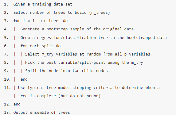
Random Forests Algorithm, from chapter 11 in (Boehmke and Greenwell 2020)
Out-of-the box performance
- Random forests tend to provide very good out-of-the-box performance, that is:
- Although several hyperparameters can be tuned,
- Default values tend to produce good results.
- Moreover, among the more popular machine learning algorithms, RFs have the least variability in their prediction accuracy when tuning (Probst, Wright, and Boulesteix 2019).
Out of the box performance
- A random forest trained with all hyperparameters set to their default values can yield an OOB RMSE that is better than many other classifiers, with or without tuning.
- This combined with good stability and ease-of-use has made it the option of choice for many problems.
Out of the box performance example
# number of features
n_features <- length(setdiff(names(ames_train), "Sale_Price"))

# train a default random forest model
ames_rf1 <- ranger(
  Sale_Price ~ .,
  data = ames_train,
  mtry = floor(n_features / 3),
  respect.unordered.factors = "order",
  seed = 123
)

# get OOB RMSE
(default_rmse <- sqrt(ames_rf1$prediction.error))
## [1] 24859.27
Tuning hyperparameters
There are several parameters that, appropriately tuned, can improve RF performance.
- Number of trees in the forest.
- Number of features to consider at any given split (\(m_{try}\)).
- Complexity of each tree.
- Sampling scheme.
- Splitting rule to use during tree construction.
1 & 2 usually have largest impact on predictive accuracy.
Random forests in bioinformatics
- Random forests have been thoroughly used in Bioinformatics (Boulesteix et al. 2012).
- Bioinformatics data are often high dimensional with
- dozens or (less often) hundreds of samples/individuals
- thousands (or hundreds of thousands) of variables.
Application of Random forests
- Random forests provide robust classifiers for:
- Distinguishing cancer from non cancer,
- Predicting tumor type in cancer of unknown origin,
- Selecting variables (SNPs) in Genome Wide Association Studies…
- Some variation of Random forests are used only for variable selection
Support Vector Machines
A Support Vector Machine (SVM) is a discriminative classifier which
intakes training data and,
outputs an optimal hyperplane
which categorizes new examples.
Linear separability
Data are said to be linearly separable if one can draw a line (plane, etc.) that separates well the groups
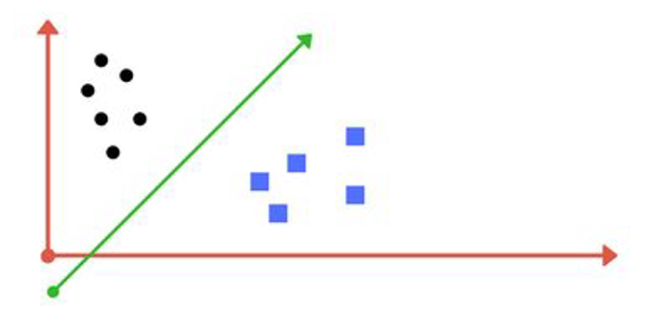
Linear vs non linear separability
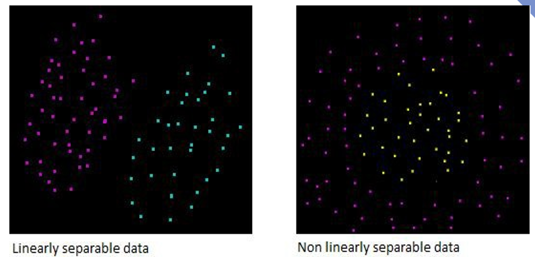
Making data separable
Projecting the data in a high-er dimensional space can turn it from non-separable to separable.
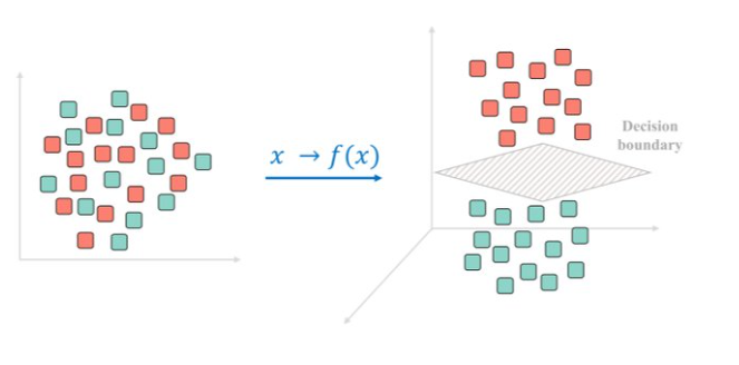
Finding the separating hyperplane
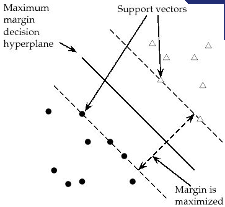
For a binary classification problem, the goal of SVM is to find the hyperplane that best separates the data points of the two classes.
This separation should maximize the margin, which is the distance between the hyperplane and the nearest data points from each class.
These nearest points are called support vectors.
Maximizing the margins
Parameters (1): Regularization
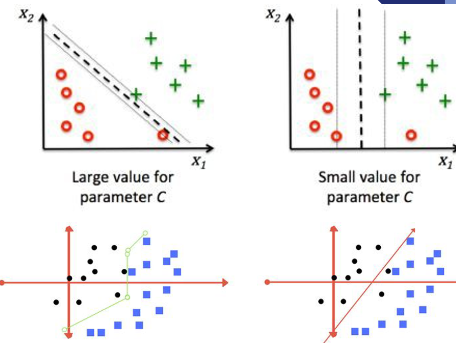
Purpose: Controls the trade-off between maximizing the margin and minimizing classification error.
Effect:
- Low C: Larger margin, more misclassifications;
- High C: Smaller margin, fewer misclassifications.
Parameters (2): Kernel
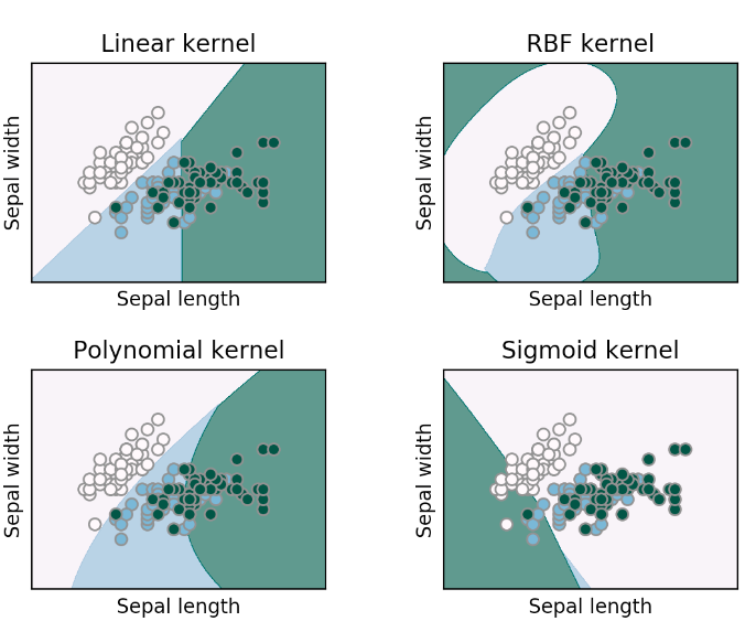
Purpose: Defines the hyperplane type for separation.
Types & Effect:
- Linear: For linearly separable data.
- Polynomial: Adds polynomial terms for non-linear data.
- RBF: Maps to higher dimensions for complex non-linear data.
Parameters (3): Gamma
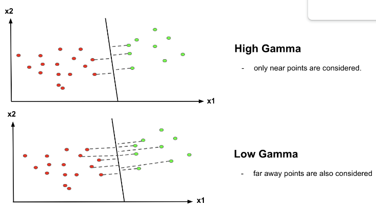
Purpose: Controls the influence of a single training example.
Effect:
- Low : Broad influence;
- High: Narrow influence.
References and Resources
References
Efron, B., Hastie T. (2016) Computer Age Statistical Inference. Cambridge University Press. Web site
Hastie, T., Tibshirani, R., & Friedman, J. (2009). The elements of statistical learning: Data mining, inference, and prediction. Springer.
James, G., Witten, D., Hastie, T., & Tibshirani, R. (2013). An introduction to statistical learning (Vol. 112). Springer. Web site
Complementary references
Breiman, L., Friedman, J., Stone, C. J., & Olshen, R. A. (1984). Classification and regression trees. CRC press.
Brandon M. Greenwell (202) Tree-Based Methods for Statistical Learning in R. 1st Edition. Chapman and Hall/CRC DOI: https://doi.org/10.1201/9781003089032
Genuer R., Poggi, J.M. (2020) Random Forests with R. Springer ed. (UseR!)
Resources
Applied Data Mining and Statistical Learning (Penn Statte-University)
An Introduction to Recursive Partitioning Using the RPART Routines
