Introduction to Keras - Lab

Introduction

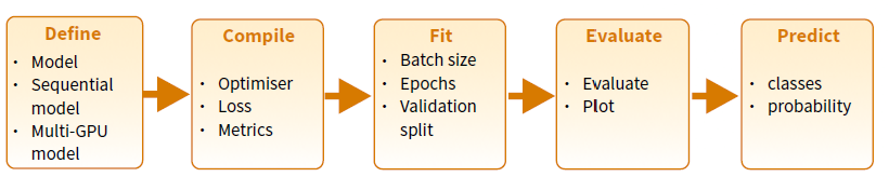
This lab has been adapted from the first lab in the Workshop on Deep learning with keras and Tensorflow in R (Rstudio conf. 2020), and has been downladed and re-created to ensure its usability.

The lab is oriented to provide a first contact with Keras in R and presents the main steps required for building training and using a deepl learning model using Keras and R as summarized in the Keras Cheatshhet:

knitr::include_graphics("images/kerasPipeline.png")

The following steps provide a good mental model for tuning a model.

It is important to recall that though they don’t guarantee you’ll find the optimal model; however, it should give you a higher probability of finding a near optimal one.

1. Prepare data
2. Balance batch size with a default learning rate
3. Tune the adaptive learning rate optimizer
4. Add callbacks to control training
5. Explore model capacity
6. Regularize overfitting
7. Repeat steps 1-6
8. Evaluate final model results

We’ll demonstrate with one of the most famous benchmark data sets, MNIST. We’ll work with a multi-layer perceptron (MLP), but realize that these steps also translate to other DL models (i.e. CNNs, RNNs, LSTMs).

Package Requirements

library(keras)       # for modeling
library(tidyverse)   # for wrangling & visualization
library(glue)        # for string literals
library(reticulate)  # Interface to 'Python'

MNIST

keras has many built in data sets (or functions to automatically install data sets). Check out the available datasets with dataset_ + tab.

We’re going to use the MNIST data set which is the “hello world” for learning deep learning! ℹ️

mnist <- dataset_mnist()
str(mnist)

List of 2
 $ train:List of 2
  ..$ x: int [1:60000, 1:28, 1:28] 0 0 0 0 0 0 0 0 0 0 ...
  ..$ y: int [1:60000(1d)] 5 0 4 1 9 2 1 3 1 4 ...
 $ test :List of 2
  ..$ x: int [1:10000, 1:28, 1:28] 0 0 0 0 0 0 0 0 0 0 ...
  ..$ y: int [1:10000(1d)] 7 2 1 0 4 1 4 9 5 9 ...

Our training images (aka features) are stored as 3D arrays:

• 60,000 images consisting of a…
• 28x28 matrix with…
• values ranging from 0-255 representing gray scale pixel values.

# 60K images of 28x28 pixels
dim(mnist$train$x)

[1] 60000    28    28

# pixel values are gray scale ranging from 0-255
range(mnist$train$x)

[1]   0 255

Notice, however, that the labels, which indicate the “true” number associated with the image are stored as a vector, because per each image (a 2-D array of 28x28) ther is a single number.

# 60K numerical labels
dim(mnist$train$y)

[1] 60000

# integer values ranging from 0 to 9
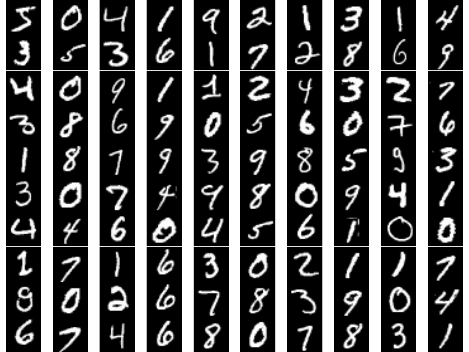
range(mnist$train$y)

[1] 0 9

Check out the first digit

digit <- mnist$train$x[1,,]
digit

      [,1] [,2] [,3] [,4] [,5] [,6] [,7] [,8] [,9] [,10] [,11] [,12] [,13]
 [1,]    0    0    0    0    0    0    0    0    0     0     0     0     0
 [2,]    0    0    0    0    0    0    0    0    0     0     0     0     0
 [3,]    0    0    0    0    0    0    0    0    0     0     0     0     0
 [4,]    0    0    0    0    0    0    0    0    0     0     0     0     0
 [5,]    0    0    0    0    0    0    0    0    0     0     0     0     0
 [6,]    0    0    0    0    0    0    0    0    0     0     0     0     3
 [7,]    0    0    0    0    0    0    0    0   30    36    94   154   170
 [8,]    0    0    0    0    0    0    0   49  238   253   253   253   253
 [9,]    0    0    0    0    0    0    0   18  219   253   253   253   253
[10,]    0    0    0    0    0    0    0    0   80   156   107   253   253
[11,]    0    0    0    0    0    0    0    0    0    14     1   154   253
[12,]    0    0    0    0    0    0    0    0    0     0     0   139   253
[13,]    0    0    0    0    0    0    0    0    0     0     0    11   190
[14,]    0    0    0    0    0    0    0    0    0     0     0     0    35
[15,]    0    0    0    0    0    0    0    0    0     0     0     0     0
[16,]    0    0    0    0    0    0    0    0    0     0     0     0     0
[17,]    0    0    0    0    0    0    0    0    0     0     0     0     0
[18,]    0    0    0    0    0    0    0    0    0     0     0     0     0
[19,]    0    0    0    0    0    0    0    0    0     0     0     0     0
[20,]    0    0    0    0    0    0    0    0    0     0     0     0    39
[21,]    0    0    0    0    0    0    0    0    0     0    24   114   221
[22,]    0    0    0    0    0    0    0    0   23    66   213   253   253
[23,]    0    0    0    0    0    0   18  171  219   253   253   253   253
[24,]    0    0    0    0   55  172  226  253  253   253   253   244   133
[25,]    0    0    0    0  136  253  253  253  212   135   132    16     0
[26,]    0    0    0    0    0    0    0    0    0     0     0     0     0
[27,]    0    0    0    0    0    0    0    0    0     0     0     0     0
[28,]    0    0    0    0    0    0    0    0    0     0     0     0     0
      [,14] [,15] [,16] [,17] [,18] [,19] [,20] [,21] [,22] [,23] [,24] [,25]
 [1,]     0     0     0     0     0     0     0     0     0     0     0     0
 [2,]     0     0     0     0     0     0     0     0     0     0     0     0
 [3,]     0     0     0     0     0     0     0     0     0     0     0     0
 [4,]     0     0     0     0     0     0     0     0     0     0     0     0
 [5,]     0     0     0     0     0     0     0     0     0     0     0     0
 [6,]    18    18    18   126   136   175    26   166   255   247   127     0
 [7,]   253   253   253   253   253   225   172   253   242   195    64     0
 [8,]   253   253   253   253   251    93    82    82    56    39     0     0
 [9,]   253   198   182   247   241     0     0     0     0     0     0     0
[10,]   205    11     0    43   154     0     0     0     0     0     0     0
[11,]    90     0     0     0     0     0     0     0     0     0     0     0
[12,]   190     2     0     0     0     0     0     0     0     0     0     0
[13,]   253    70     0     0     0     0     0     0     0     0     0     0
[14,]   241   225   160   108     1     0     0     0     0     0     0     0
[15,]    81   240   253   253   119    25     0     0     0     0     0     0
[16,]     0    45   186   253   253   150    27     0     0     0     0     0
[17,]     0     0    16    93   252   253   187     0     0     0     0     0
[18,]     0     0     0     0   249   253   249    64     0     0     0     0
[19,]     0    46   130   183   253   253   207     2     0     0     0     0
[20,]   148   229   253   253   253   250   182     0     0     0     0     0
[21,]   253   253   253   253   201    78     0     0     0     0     0     0
[22,]   253   253   198    81     2     0     0     0     0     0     0     0
[23,]   195    80     9     0     0     0     0     0     0     0     0     0
[24,]    11     0     0     0     0     0     0     0     0     0     0     0
[25,]     0     0     0     0     0     0     0     0     0     0     0     0
[26,]     0     0     0     0     0     0     0     0     0     0     0     0
[27,]     0     0     0     0     0     0     0     0     0     0     0     0
[28,]     0     0     0     0     0     0     0     0     0     0     0     0
      [,26] [,27] [,28]
 [1,]     0     0     0
 [2,]     0     0     0
 [3,]     0     0     0
 [4,]     0     0     0
 [5,]     0     0     0
 [6,]     0     0     0
 [7,]     0     0     0
 [8,]     0     0     0
 [9,]     0     0     0
[10,]     0     0     0
[11,]     0     0     0
[12,]     0     0     0
[13,]     0     0     0
[14,]     0     0     0
[15,]     0     0     0
[16,]     0     0     0
[17,]     0     0     0
[18,]     0     0     0
[19,]     0     0     0
[20,]     0     0     0
[21,]     0     0     0
[22,]     0     0     0
[23,]     0     0     0
[24,]     0     0     0
[25,]     0     0     0
[26,]     0     0     0
[27,]     0     0     0
[28,]     0     0     0

Lets plot the first digit and compare to the above matrix.

plot(as.raster(digit, max = 255))

The associated label confirms it is number 5.

mnist$train$y[1]

[1] 5

Now lets check out the first 100 digits

par(mfrow = c(10, 10), mar = c(0,0,0,0))
for (i in 1:100) {
  plot(as.raster(mnist$train$x[i,,], max = 255))
}

Prepare Data

When we work with keras:

• training and test sets need to be independent
• features and labels (aka target, response) need to be independent
• use %<-% for object unpacking (see ?zeallot::%<-%)

c(c(train_images, train_labels), c(test_images, test_labels)) %<-% mnist

# the above is the same as
# train_images <- mnist$train$x
# train_labels <- mnist$train$y
# test_images <- mnist$test$x
# test_labels <- mnist$test$y

Shape into proper tensor form

The shape of our data is dependent on the type of DL model we are training. Multi Layer Perceptrons (MLPs) require our data to be in a 2D tensor (aka matrix); however, our data are currently in a 3D tensor.

We can reshape our tensor from 3D to 2D. Much like a matrix can be flattened to a vector:

m <- matrix(1:9, nrow = 3)
m

     [,1] [,2] [,3]
[1,]    1    4    7
[2,]    2    5    8
[3,]    3    6    9

# flattened matrix
as.vector(m)

[1] 1 2 3 4 5 6 7 8 9

# Warning of how you invert the process !!!
# matrix(as.vector(m), nrow=3)

We can reshape a 3D array to a 2D array with array_reshape()

knitr::include_graphics("images/reshape.png")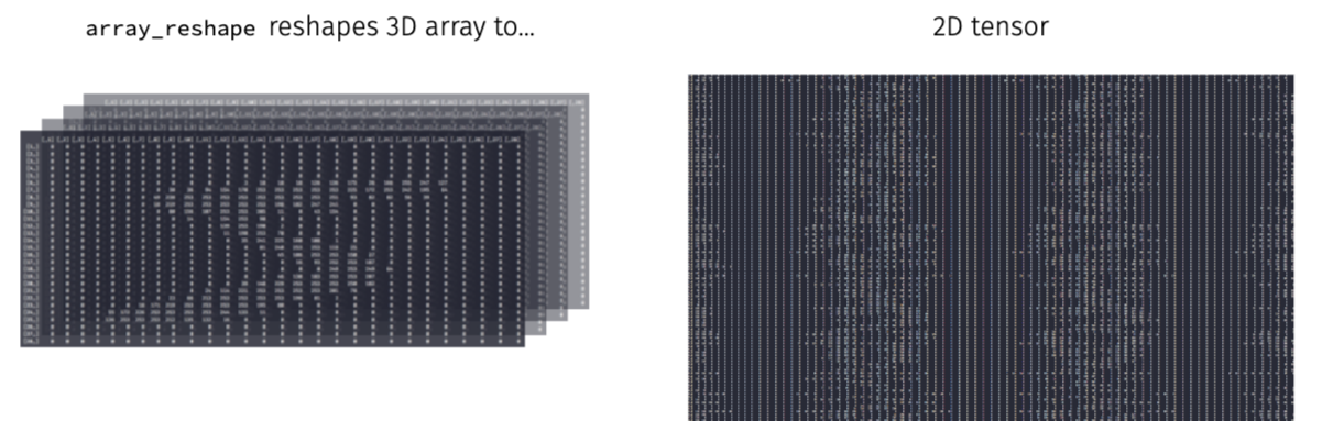

# reshape 3D tensor (aka array) to a 2D tensor (aka matrix)
train_images <- array_reshape(train_images, c(60000, 28 * 28))
test_images <- array_reshape(test_images, c(10000, 28 * 28))

# our training data is now a matrix with 60K observations and
# 784 features (28 pixels x 28 pixels = 784)
str(train_images)

 num [1:60000, 1:784] 0 0 0 0 0 0 0 0 0 0 ...

Since we are dealing with a multi-classification problem where the target ranges from 0-9, we’ll reformat the labels with to_categorical().

This function takes a vector of \(N\) integers of \(k\) distinct classes and creates a matrix of \(N\) rows and \(k\) columns in such a way that if the nth value in the original vector, was a 7, now the nth row, column 8, in the transformed matrix, has a 1 and the remaining columns of this row contain a zero.

Note: column 1 refers to the digit “0”, column 2 refers to the digit “1”, etc.

class(train_labels)

[1] "array"

dim(train_labels)

[1] 60000

train_labels <- to_categorical(train_labels)
test_labels <- to_categorical(test_labels)
class(train_labels)

[1] "matrix" "array" 

dim(train_labels)

[1] 60000    10

head(train_labels)

     [,1] [,2] [,3] [,4] [,5] [,6] [,7] [,8] [,9] [,10]
[1,]    0    0    0    0    0    1    0    0    0     0
[2,]    1    0    0    0    0    0    0    0    0     0
[3,]    0    0    0    0    1    0    0    0    0     0
[4,]    0    1    0    0    0    0    0    0    0     0
[5,]    0    0    0    0    0    0    0    0    0     1
[6,]    0    0    1    0    0    0    0    0    0     0

Stabilize learning by data scaling

When applying DL models, our feature values should not be relatively large compared to the randomized initial weights and all our features should take values in roughly the same range.

When features have large or widely varying values, large gradient updates can be triggered that will prevent the network from converging

Tips:

1. When all features have the same value range (i.e. images), we can standardize values between 0-1.

2. When features varying in range from one another (i.e. age, height, longitude) normalize each feature to have mean of 0 and standard deviation of 1 (?scale())

# all our features (pixels) range from 0-255
range(train_images)

[1]   0 255

# standardize train and test features
train_images <- train_images / 255
test_images <- test_images / 255

Randomize data

Although this dataset is not ordered, it is a good practice to randomize data so that our train and validation datasets are properly represented.

obs <- nrow(train_images)
set.seed(123)
randomize <- sample(seq_len(obs), size = obs, replace = FALSE)
train_images <- train_images[randomize, ]
train_labels <- train_labels[randomize, ]

Once the data has been prepared we can proceed to train some DL models!!

Balance Batch Size & Default Learning Rate

Terms recall: Batch, Epoch, Learning rate.

• Epoch: A complete pass through the entire training dataset.

  • Example: Training a model on 1,000 images where each image is seen once.

• Batch: A subset of the training dataset used to update the model’s parameters.

  • Example: Processing 100 images at a time during training.

• Mini-batch: A smaller subset of the training dataset used for parameter updates.

  • Example: Processing 32 images at a time during training with limited memory.

The learning rate is the most important hyperparameter to get right but before I tuning it, I like to find a batch size that balances:

• smoothness of the learning curve
• speed of training

Tips: start with…

• a default learning rate,
• a single hidden layer with units set to around mean(n_features + n_response_classes),
• the default batch size of 32,
• then test ranges of batch sizes [16, 32, 64, 128, 256, 512].

# get number of features
n_feat <- ncol(train_images)

# 1. Define model architecture
model <- keras_model_sequential() %>%
  layer_dense(units = 512, activation = 'relu', 
              input_shape = n_feat) %>%
  layer_dense(units = 10, activation = 'softmax')

# 1. Define model architecture
model <- keras_model_sequential() %>%
  layer_dense(units = 512, activation = 'relu', input_shape = c(n_feat)) %>%
  layer_dense(units = 10, activation = 'softmax')


# 2. Define how our model is going to learn
model %>% compile(
  loss = "categorical_crossentropy",
  optimizer = "sgd",
  metrics = "accuracy"
)

summary(model)

Model: "sequential_1"
________________________________________________________________________________
 Layer (type)                       Output Shape                    Param #     
================================================================================
 dense_3 (Dense)                    (None, 512)                     401920      
 dense_2 (Dense)                    (None, 10)                      5130        
================================================================================
Total params: 407,050
Trainable params: 407,050
Non-trainable params: 0
________________________________________________________________________________

Let’s train our model with the default batch size of 32.

# 3. Train our model
history <- model %>% fit(
  train_images, train_labels,
  validation_split = 0.2
  )

history

Final epoch (plot to see history):
        loss: 0.1699
    accuracy: 0.953
    val_loss: 0.1778
val_accuracy: 0.9486 

plot(history)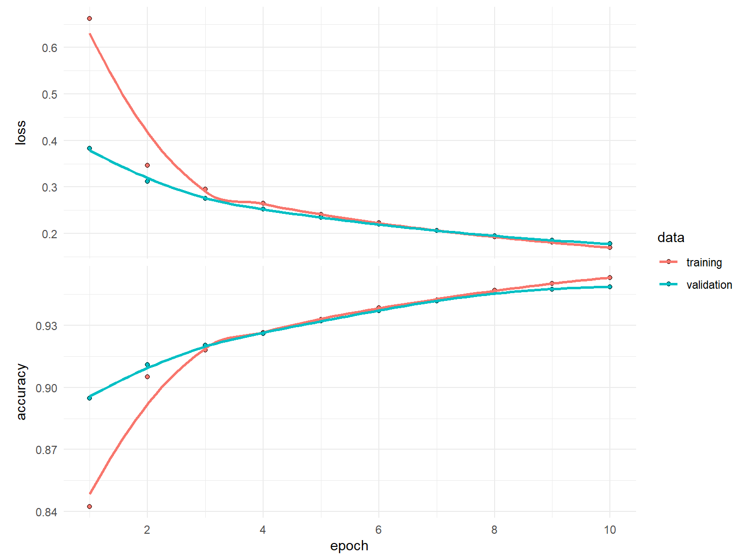

Your turn! (3min)

Now retrain the same model but try with batch sizes of 16, 128, 512 while leaving everything else the same. How do the results (loss, accuracy, and compute time) compare?

# define model architecture
model <- keras_model_sequential() %>%
  layer_dense(units = 512, activation = 'relu', input_shape = n_feat) %>%
  layer_dense(units = 10, activation = 'softmax')

# define how the model is gonig to learn
model %>% compile(
  loss = "categorical_crossentropy",
  optimizer = "sgd",
  metrics = "accuracy"
  )

history <- model %>% fit(
  train_images, train_labels,
  validation_split = 0.2,
  ____ = ____
  )

Pick an Adaptive Learning Rate Optimizer

Once we’ve picked an adequate batch size, next we want to start tuning the learning rate. There are two main considerations:

1. We usually always assess different learning rates ranging from [1e-1, 1e-7].
2. Adaptive learning rate optimizers nearly always outperform regular SGD

Adaptive learning rates help to escape “saddle points”.

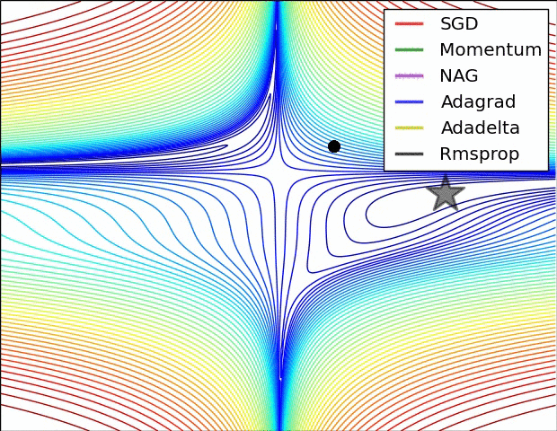
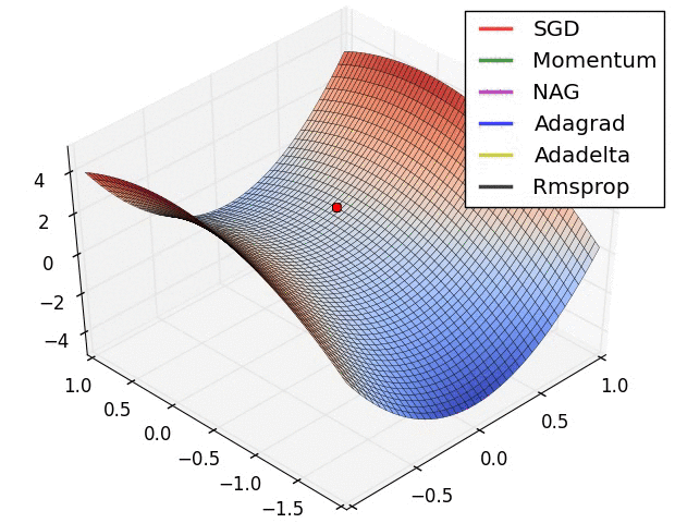
The primary adaptive learning rates include:

1. SGD (Stochastic Gradient Descent): Basic optimization algorithm that updates model parameters based on the negative gradient of the loss function.

2. SGD with momentum: Extends SGD by incorporating a momentum term, which helps accelerate learning and maintain direction in the presence of noisy or sparse gradients.

3. nAG (Nesterov Accelerated Gradient): Variant of SGD that improves convergence speed by calculating the gradient at a lookahead position, providing more accurate gradient information.

4. Adagrad (Adaptive Gradient): Adapts the learning rate for each parameter based on the historical gradients, giving more weight to parameters with smaller gradients.

5. Adadelta: Extension of Adagrad that dynamically adjusts the learning rate using the ratio of accumulated gradients to accumulated parameter updates.

6. RMSprop (Root Mean Square Propagation): Adaptive learning rate algorithm that normalizes learning rates by dividing them by an exponentially weighted moving average of squared gradients.

These optimization techniques offer different strategies for updating model parameters, improving convergence and adapting the learning rate to optimize model performance.

See ?optimizer_sgd() or ?optimizer_rmsprop()

See https://ruder.io/optimizing-gradient-descent/ for more details

Your turn! (5min)

Retrain our DL model using:

• SGD with momentum (optimizer_sgd())
  • Try default learning rate (0.01) with momentum (0.5, 0.9, 0.99)
  • Try larger learning rates (0.1, 1) with momentum
• RMSprop (optimizer_rmsprop())
  • What is the default learning rate? Train with default.
  • Try a larger learning rate. What happens?
• Adam (optimizer_adam())
  • What is the default learning rate? Train with default.
  • Try a larger learning rate. What happens?

model <- keras_model_sequential() %>%
  layer_dense(units = 512, activation = 'relu', input_shape = n_feat) %>%
  layer_dense(units = 10, activation = 'softmax')

model %>% compile(
  loss = "categorical_crossentropy",
  optimizer = ____,
  metrics = "accuracy"
  )

history <- model %>% fit(
  train_images, train_labels,
  validation_split = 0.2,
  batch_size = 128
  )

Add Callbacks

When training a model, sometimes we want to:

• automatically stop a model once performance has stopped improving
• dynamically adjust values of certain parameters (i.e. learning rate)
• log model information to use or visualize later on
• continually save the model during training and save the model with the best performance

Keras provides a suite of tools called _callbacks that help us to monitor, control, and customize the training procedure.

Stop training at the right time

We often don’t know how many epochs we’ll need to reach a minimum loss. The early stopping callback allows us to automatically stop training after we experience no improvement in our loss after patience number of epochs.

• If you are going to use the model after training you always want to retain the “best” model, which is the model with the lowest loss. restore_best_weights will restore the weights for this “best” model even after you’ve passed it by n epochs.

• Sometimes your model will stall on a low validation loss resulting in a tie. Even with early stopping the model will continue to train for all the epochs. min_delta allows you to state some small value that the loss must improve by otherwise it will stop.

model <- keras_model_sequential() %>%
  layer_dense(units = 512, activation = 'relu', input_shape = n_feat) %>%
  layer_dense(units = 10, activation = 'softmax')

model %>% compile(
  loss = "categorical_crossentropy",
  optimizer = optimizer_sgd(learning_rate = 0.1, 
                            momentum = 0.9),
  metrics = "accuracy"
)

history <- model %>% fit(
  train_images, train_labels,
  validation_split = 0.2,
  batch_size = 128,
  epochs = 20,
  callback = callback_early_stopping(patience = 3,
            restore_best_weights = TRUE,
            min_delta = 0.0001)
  )

history

Final epoch (plot to see history):
        loss: 0.003236
    accuracy: 0.9998
    val_loss: 0.06499
val_accuracy: 0.9832 

Note how we did not train for all the epochs…only until our loss didn’t improve by 0.0001 for 3 consistent epochs.

plot(history)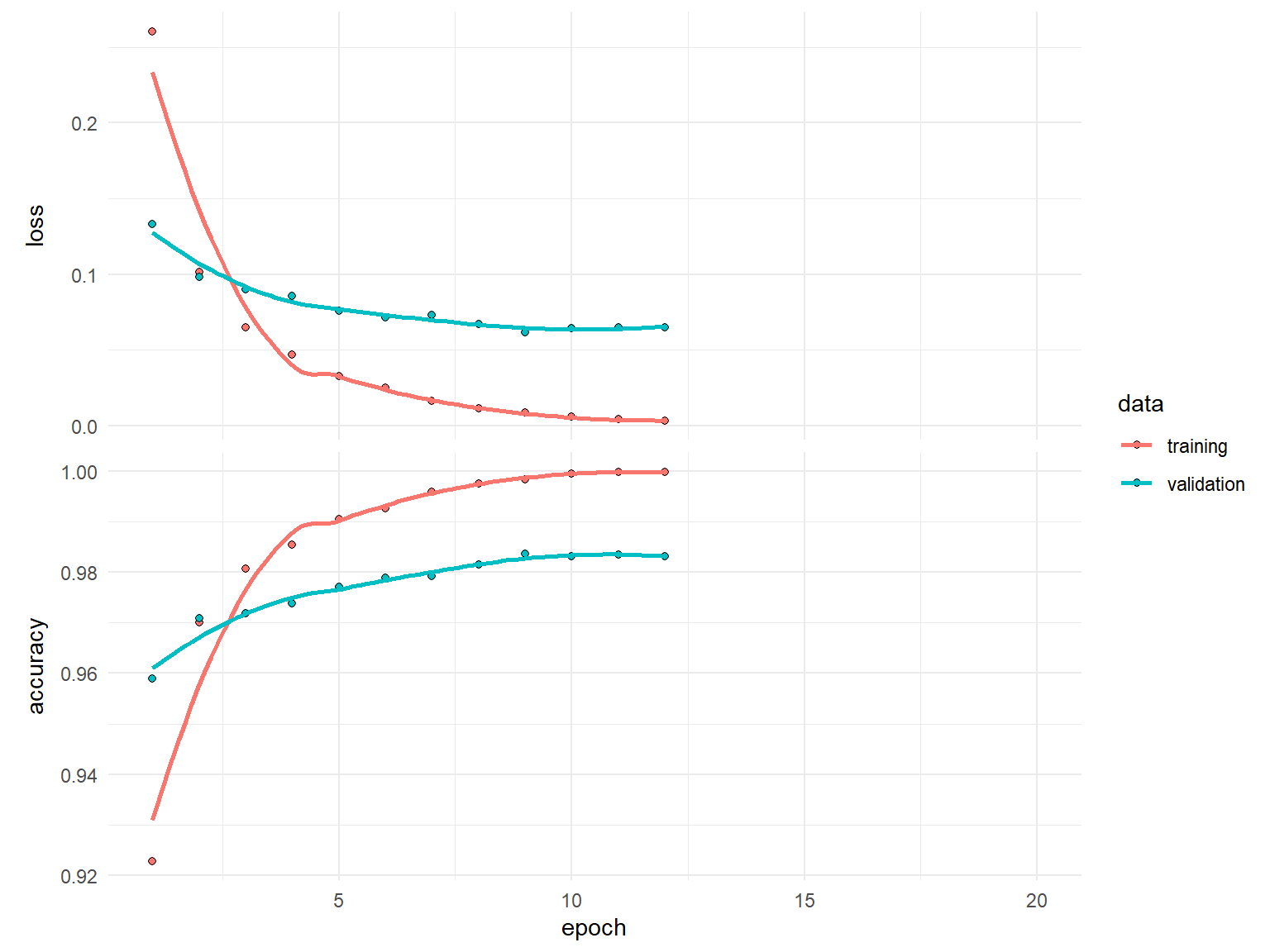

Add a learning rate scheduler

Although adaptive learning rate optimizers adjust the velocity of weight updates depending on the loss surface, we can also incorporate additional ways to modify the learning rate “on the fly”.

• Learning rate decay reduces the learning rate at each epoch. Note the decay argument in ?optimizer_xxx().

• There has been some great research on cyclical learning rates (see https://arxiv.org/abs/1506.01186). You can incorporate custom learning rates such as this with callback_learning_rate_scheduler(). This is more advanced but definitely worth reading.

• A simpler, and very practical approach, is to reduce the learning rate after the model has stopped improving with callback_reduce_lr_on_plateau(). This approach allows the model to tell us when to reduce the learning rate.

When using decay or callback_reduce_lr_on_plateau(), you can usually increase the base learning rate so that you learn quickly early on and then the learning rate will reduce so you can take smaller steps as you approach the minimum loss.

model <- keras_model_sequential() %>%
  layer_dense(units = 512, activation = 'relu', input_shape = n_feat) %>%
  layer_dense(units = 10, activation = 'softmax')

model %>% compile(
  loss = "categorical_crossentropy",
  optimizer = optimizer_sgd(learning_rate = 0.1, momentum = 0.9),
  metrics = "accuracy"
)

history <- model %>% fit(
  train_images, train_labels,
  validation_split = 0.2,
  batch_size = 128,
  epochs = 20,
  callback = list(
    callback_early_stopping(patience = 3, restore_best_weights = TRUE, min_delta = 0.0001),
    callback_reduce_lr_on_plateau(patience = 1, factor = 0.1)
    )
  )

history

Final epoch (plot to see history):
        loss: 0.007838
    accuracy: 0.9994
    val_loss: 0.06073
val_accuracy: 0.9835
          lr: 0.0001 

plot(history)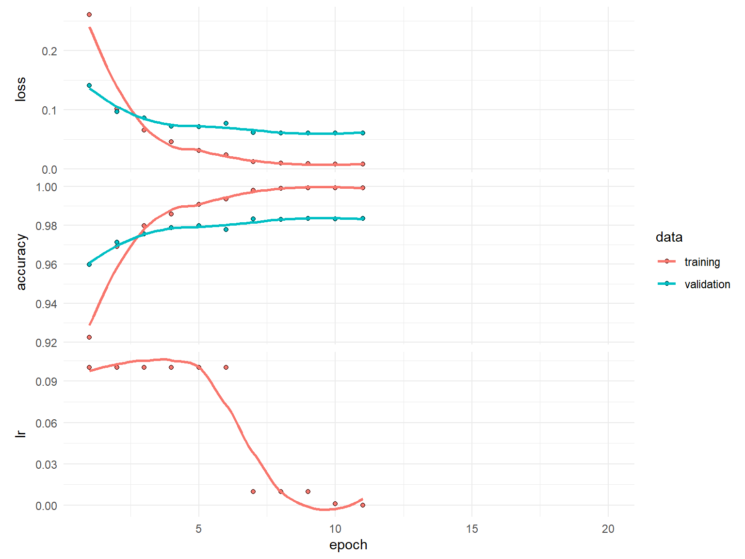

plot(history$metrics$lr)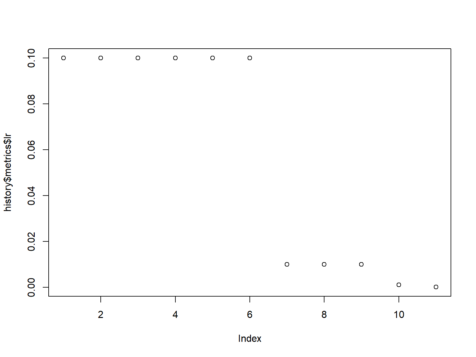

Explore Model Capacity

Now that we have found a pretty good learning rate and we have good control over our training procedure with callbacks, we can start to assess how the capacity of our model effects performance.

The capacity of a deep learning model refers to its ability to learn complex patterns in the data.

It is determined by the architecture, including the number of layers and neurons.

Higher capacity allows the model to capture more intricate details, but it also increases the risk of overfitting.

Finding the right balance is important for optimal performance.

Capacity is usually controlled in two ways:

• width: the number of units in a hidden layer
• depth: the number of hidden layers

Your turn! (5min)

Explore different model capacities while all other parameters constant. Try increasing

• Width: remember that the number of units is usually a power of 2 (i.e. 32, 64, 128, 256, 512, 1024).
• Depth: try using 2 or 3 hidden layers

model <- keras_model_sequential() %>%
  ___________ %>%
  layer_dense(units = 10, activation = 'softmax')

model %>% compile(
  loss = "categorical_crossentropy",
  optimizer = optimizer_sgd(lr = 0.1, momentum = 0.9),
  metrics = "accuracy"
)

history <- model %>% fit(
  train_images, train_labels,
  validation_split = 0.2,
  batch_size = 128,
  epochs = 20,
  callback = list(
    callback_early_stopping(patience = 3, restore_best_weights = TRUE, min_delta = 0.0001),
    callback_reduce_lr_on_plateau(patience = 1, factor = 0.1)
    )
  )

Smart experimenting

As we start to experiment more, it becomes harder to organize and compare our results. Let’s make it more efficient by:

• Creating a function that allows us to dynamically change the number of layers and units.
• Using callback_tensorboard() which allows us to save and visually compare results.

There is another approach to performing grid searches. See the extras notebook https://rstudio-conf-2020.github.io/dl-keras-tf/notebooks/imdb-grid-search.nb.html for details.

train_model <- function(n_units, n_layers, log_to) {
  
  # Create a model with a single hidden input layer
  model <- keras_model_sequential() %>%
    layer_dense(units = n_units, activation = "relu", input_shape = n_feat)
  
  # Add additional hidden layers based on input
  if (n_layers > 1) {
    for (i in seq_along(n_layers - 1)) {
      model %>% layer_dense(units = n_units, activation = "relu")
    }
  }
  
  # Add final output layer
  model %>% layer_dense(units = 10, activation = "softmax")
  
  # compile model
  model %>% compile(
    loss = "categorical_crossentropy",
    optimizer = optimizer_sgd(learning_rate = 0.1, momentum = 0.9),
    metrics = "accuracy"
  )
  
  # train model and store results with callback_tensorboard()
  history <- model %>% fit(
    train_images, train_labels,
    validation_split = 0.2,
    batch_size = 128,
    epochs = 20,
    callback = list(
      callback_early_stopping(patience = 3, restore_best_weights = TRUE, min_delta = 0.0001),
      callback_reduce_lr_on_plateau(patience = 1, factor = 0.1),
      callback_tensorboard(log_dir = log_to)
      ),
    verbose = FALSE
    )
  
  return(history)
  }

Now we can create a grid for various model capacities. We include an ID for each model, which we will use to save our results within callback_tensorboard().

grid <- expand_grid(
  units = c(128, 256, 512, 1024),
  layers = c(1:3)
) %>%
  mutate(id = paste0("mlp_", layers, "_layers_", units, "_units"))
grid

# A tibble: 12 × 3
   units layers id                     
   <dbl>  <int> <chr>                  
 1   128      1 mlp_1_layers_128_units 
 2   128      2 mlp_2_layers_128_units 
 3   128      3 mlp_3_layers_128_units 
 4   256      1 mlp_1_layers_256_units 
 5   256      2 mlp_2_layers_256_units 
 6   256      3 mlp_3_layers_256_units 
 7   512      1 mlp_1_layers_512_units 
 8   512      2 mlp_2_layers_512_units 
 9   512      3 mlp_3_layers_512_units 
10  1024      1 mlp_1_layers_1024_units
11  1024      2 mlp_2_layers_1024_units
12  1024      3 mlp_3_layers_1024_units

Now we can loop through each model capacity combination and train our models.

This will take a few minutes so this is a good time to save your work and take a break.

system.time(
for (row in seq_len(nrow(grid))) {
  # get parameters
  units <- grid[[row, "units"]]
  layers <- grid[[row, "layers"]]
  file_path <- paste0("mnist/", grid[[row, "id"]])
  
  # provide status update
  cat(layers, "hidden layer(s) with", units, "neurons: ")
  
  # train model
  m <- train_model(n_units = units, n_layers = layers, log_to = file_path)
  min_loss <- min(m$metrics$val_loss, na.rm = TRUE)
  
  # update status with loss
  cat(min_loss, "\n", append = TRUE)
}
)

1 hidden layer(s) with 128 neurons: 0.07069184 
2 hidden layer(s) with 128 neurons: 0.06938207 
3 hidden layer(s) with 128 neurons: 0.06946184 
1 hidden layer(s) with 256 neurons: 0.06554866 
2 hidden layer(s) with 256 neurons: 0.06640807 
3 hidden layer(s) with 256 neurons: 0.07036863 
1 hidden layer(s) with 512 neurons: 0.06244506 
2 hidden layer(s) with 512 neurons: 0.06106765 
3 hidden layer(s) with 512 neurons: 0.06557445 
1 hidden layer(s) with 1024 neurons: 0.06027493 
2 hidden layer(s) with 1024 neurons: 0.05934745 
3 hidden layer(s) with 1024 neurons: 0.05973132 

   user  system elapsed 
 128.89   75.78  287.67 

Our results suggest that larger width models tend to perform better but it is unclear if deeper models add much benefit. However, to get more clarity we can analyze the learning rates with tensorboard().

Note that callback_tensorboard() saved all the model runs in /mnist subdirectory.

tensorboard("mnist")

Started TensorBoard at http://127.0.0.1:3383 

Your turn! (3 min)

Retrain the model with:

• 2 hidden layers
• 1024 units in each hidden layer
• early stopping after 3 epochs of no improvement
• reduce learning rate after 1 epoch of no improvement

model <- keras_model_sequential() %>%
  ___________ %>%
  ___________

model %>% compile(
  loss = "categorical_crossentropy",
  optimizer = optimizer_sgd(lr = 0.1, momentum = 0.9),
  metrics = "accuracy"
)

history <- model %>% fit(
  train_images, train_labels,
  validation_split = 0.2,
  batch_size = 128,
  epochs = 20,
  callback = list(
    callback______(patience = _____, restore_best_weights = TRUE, min_delta = 0.0001),
    callback______(patience = _____, factor = 0.1)
    )
  )

Regularize Overfitting

Often, once we’ve found a model that minimizes the loss, there is still some overfitting that is occuring…sometimes a lot.

So our next objective is to try flatten the validation loss learning curve and bring it as close to the training loss curve as possible.

Weight decay

A common way to mitigate overfitting is to put constraints on the complexity of a network by forcing its weights to take on small values, which makes the distribution of weight values more regular.

This is called weight regularization and its done by adding to the loss function of the network a cost associated with having large weights.

If you a familiar with regularized regression ℹ️ (lasso, ridge, elastic nets) then weight regularization is essentially the same thing. ℹ️

\[Loss = MSE + \lambda \sum^p_{j=1} w^2_j\]

• Although you can use L1, L2 or a combination, L2 is by far the most common and is known as weight decay in the context of neural nets.
• Optimal values vary but when tuning we typically start with factors of \(10^{-s}\) where s ranges between 1-4 (0.1, 0.01, …, 0.0001).
• The larger the weight regularizer, the more epochs generally required to reach a minimum loss.
• Weight decay can cause a noisier learning curve so its often beneficial to increase the patience parameter for early stopping if this is noticable.

model <- keras_model_sequential() %>%
  layer_dense(
    units = 512, activation = "relu", input_shape = n_feat,
    kernel_regularizer = regularizer_l2(l = 0.001)    # regularization parameter
    ) %>%
  layer_dense(
    units = 512, activation = "relu",
    kernel_regularizer = regularizer_l2(l = 0.001)    # regularization parameter
    ) %>%
  layer_dense(units = 10, activation = "softmax")

model %>% compile(
  loss = "categorical_crossentropy",
  optimizer = optimizer_sgd(learning_rate = 0.1, 
                            momentum = 0.9),
  metrics = "accuracy"
)

history <- model %>% fit(
  train_images, train_labels,
  validation_split = 0.2,
  batch_size = 128,
  epochs = 20,
  callback = list(
    callback_early_stopping(patience = 3, restore_best_weights = TRUE, min_delta = 0.0001),
    callback_reduce_lr_on_plateau(patience = 1, factor = 0.1)
    )
  )

history

Final epoch (plot to see history):
        loss: 0.09333
    accuracy: 0.996
    val_loss: 0.1284
val_accuracy: 0.9823
          lr: 0.001 

plot(history)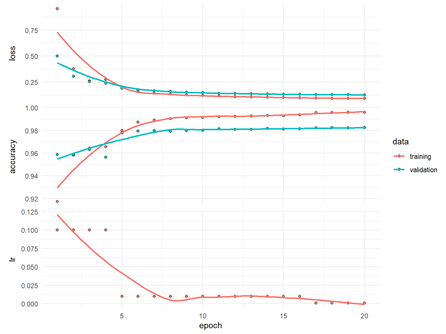

Dropout

Dropout is one of the most effective and commonly used regularization techniques for neural networks.

Dropout applied to a layer randomly drops out (sets to zero) a certain percentage of the output features of that layer.

By randomly dropping some of a layer’s outputs we minimize the chance of fitting patterns to noise in the data, a common cause of overfitting.

• Dropout rates typically ranges between 0.2-0.5. Sometimes higher rates are necessary but note that you will get a warning when supplying rate > 0.5.

• The higher the dropout rate, the slower the convergence so you may need to increase the number of epochs.

• Its common to apply dropout after each hidden layer and with the same rate;

• however, this is not necessary.

model <- keras_model_sequential() %>%
  layer_dense(units = 512, activation = "relu", input_shape = n_feat) %>%
  layer_dropout(0.3) %>%                            # regularization parameter
  layer_dense(units = 512, activation = "relu") %>%
  layer_dropout(0.3) %>%                           # regularization parameter
  layer_dense(units = 10, activation = "softmax")

model %>% compile(
  loss = "categorical_crossentropy",
  optimizer = optimizer_sgd(learning_rate = 0.1, 
                            momentum = 0.9),
  metrics = "accuracy"
)

history <- model %>% fit(
  train_images, train_labels,
  validation_split = 0.2,
  batch_size = 128,
  epochs = 20,
  callback = list(
    callback_early_stopping(patience = 3, restore_best_weights = TRUE, min_delta = 0.0001),
    callback_reduce_lr_on_plateau(patience = 1, factor = 0.1)
    )
  ) %>%
  as.data.frame()

history

    epoch        value   metric       data
1       1 3.242483e-01     loss   training
2       2 1.482577e-01     loss   training
3       3 1.137299e-01     loss   training
4       4 9.758937e-02     loss   training
5       5 7.881726e-02     loss   training
6       6 6.788949e-02     loss   training
7       7 6.261241e-02     loss   training
8       8 4.050179e-02     loss   training
9       9 3.128683e-02     loss   training
10     10 2.672179e-02     loss   training
11     11 2.508097e-02     loss   training
12     12 2.197508e-02     loss   training
13     13 2.042278e-02     loss   training
14     14 2.059718e-02     loss   training
15     15           NA     loss   training
16     16           NA     loss   training
17     17           NA     loss   training
18     18           NA     loss   training
19     19           NA     loss   training
20     20           NA     loss   training
21      1 8.989375e-01 accuracy   training
22      2 9.537917e-01 accuracy   training
23      3 9.648333e-01 accuracy   training
24      4 9.694791e-01 accuracy   training
25      5 9.750834e-01 accuracy   training
26      6 9.785417e-01 accuracy   training
27      7 9.797083e-01 accuracy   training
28      8 9.865834e-01 accuracy   training
29      9 9.901250e-01 accuracy   training
30     10 9.915208e-01 accuracy   training
31     11 9.917708e-01 accuracy   training
32     12 9.930000e-01 accuracy   training
33     13 9.931250e-01 accuracy   training
34     14 9.934375e-01 accuracy   training
35     15           NA accuracy   training
36     16           NA accuracy   training
37     17           NA accuracy   training
38     18           NA accuracy   training
39     19           NA accuracy   training
40     20           NA accuracy   training
41      1 1.419821e-01     loss validation
42      2 1.198308e-01     loss validation
43      3 9.774947e-02     loss validation
44      4 8.783271e-02     loss validation
45      5 8.001570e-02     loss validation
46      6 7.208887e-02     loss validation
47      7 7.537550e-02     loss validation
48      8 6.350064e-02     loss validation
49      9 6.203371e-02     loss validation
50     10 6.138184e-02     loss validation
51     11 6.125287e-02     loss validation
52     12 6.218536e-02     loss validation
53     13 6.142388e-02     loss validation
54     14 6.137693e-02     loss validation
55     15           NA     loss validation
56     16           NA     loss validation
57     17           NA     loss validation
58     18           NA     loss validation
59     19           NA     loss validation
60     20           NA     loss validation
61      1 9.568334e-01 accuracy validation
62      2 9.630000e-01 accuracy validation
63      3 9.705000e-01 accuracy validation
64      4 9.735833e-01 accuracy validation
65      5 9.779167e-01 accuracy validation
66      6 9.800833e-01 accuracy validation
67      7 9.792500e-01 accuracy validation
68      8 9.827500e-01 accuracy validation
69      9 9.837500e-01 accuracy validation
70     10 9.838333e-01 accuracy validation
71     11 9.838333e-01 accuracy validation
72     12 9.841667e-01 accuracy validation
73     13 9.843333e-01 accuracy validation
74     14 9.843333e-01 accuracy validation
75     15           NA accuracy validation
76     16           NA accuracy validation
77     17           NA accuracy validation
78     18           NA accuracy validation
79     19           NA accuracy validation
80     20           NA accuracy validation
81      1 1.000000e-01       lr   training
82      2 1.000000e-01       lr   training
83      3 1.000000e-01       lr   training
84      4 1.000000e-01       lr   training
85      5 1.000000e-01       lr   training
86      6 1.000000e-01       lr   training
87      7 1.000000e-01       lr   training
88      8 1.000000e-02       lr   training
89      9 1.000000e-02       lr   training
90     10 1.000000e-02       lr   training
91     11 1.000000e-02       lr   training
92     12 1.000000e-02       lr   training
93     13 9.999999e-04       lr   training
94     14 9.999999e-05       lr   training
95     15           NA       lr   training
96     16           NA       lr   training
97     17           NA       lr   training
98     18           NA       lr   training
99     19           NA       lr   training
100    20           NA       lr   training

plot(history)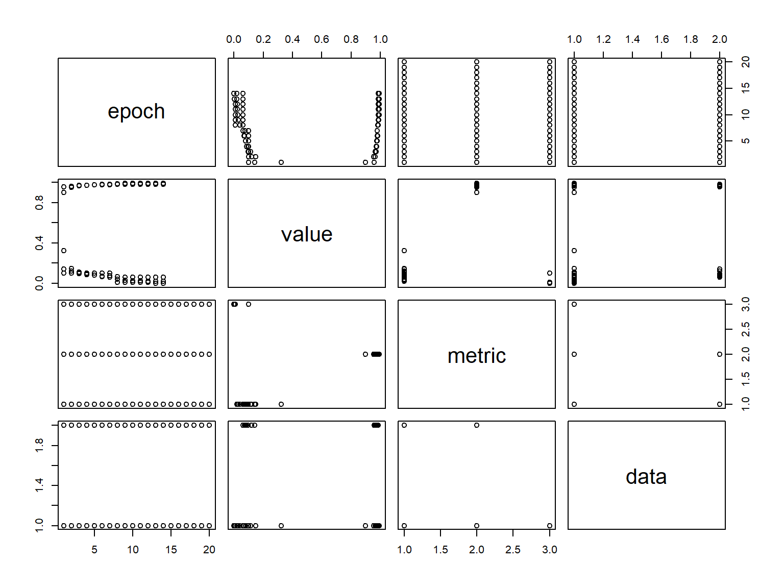

Repeat

At this point, we have a pretty good model. However, often, iterating over these steps can improve model performance even further. For brevity, we’ll act as if we have found a sufficient solution.

Evaluate results

Once a final model is chosen, we can evaluate the model on our test set to provide us with a accurate expectation of our generalization error. Our goal is that our test error is very close to our validation error.

model %>% evaluate(test_images, test_labels, verbose = FALSE)

      loss   accuracy 
0.05530928 0.98350000 

Confusion matrix

To understand our model’s performance across the different response classes, we can assess a confusion matrix ℹ️.

First, we need to predict our classes and also get the actual response values.

predictions <- model %>% predict(test_images) %>% k_argmax()
actual <- mnist$test$y

We can see the number of missed predictions in our test set

library(reticulate)
predictions <- as.array(predictions)
missed_predictions <- sum(predictions != actual)
missed_predictions

[1] 165

We can use caret::confusionMatrix() to get our confusion matrix. We can see which digits our model confuses the most by analyzing the confusion matrix.

• 9s are often confused with 4s
• 6s are often confused with 0s & 5s
• etc.

caret::confusionMatrix(factor(predictions), factor(actual))

Confusion Matrix and Statistics

          Reference
Prediction    0    1    2    3    4    5    6    7    8    9
         0  971    0    4    0    1    2    3    1    4    1
         1    1 1128    0    0    1    0    3    5    0    2
         2    0    1 1017    4    2    0    0    7    3    0
         3    0    2    2  993    1    7    0    1    3    3
         4    1    0    1    0  965    0    3    0    1    9
         5    0    1    1    4    0  874    7    0    3    2
         6    3    2    2    0    3    2  940    0    2    1
         7    1    0    3    3    1    1    1 1009    3    4
         8    2    1    2    5    2    2    1    2  952    1
         9    1    0    0    1    6    4    0    3    3  986

Overall Statistics
                                          
               Accuracy : 0.9835          
                 95% CI : (0.9808, 0.9859)
    No Information Rate : 0.1135          
    P-Value [Acc > NIR] : < 2.2e-16       
                                          
                  Kappa : 0.9817          
                                          
 Mcnemar's Test P-Value : NA              

Statistics by Class:

                     Class: 0 Class: 1 Class: 2 Class: 3 Class: 4 Class: 5
Sensitivity            0.9908   0.9938   0.9855   0.9832   0.9827   0.9798
Specificity            0.9982   0.9986   0.9981   0.9979   0.9983   0.9980
Pos Pred Value         0.9838   0.9895   0.9836   0.9812   0.9847   0.9798
Neg Pred Value         0.9990   0.9992   0.9983   0.9981   0.9981   0.9980
Prevalence             0.0980   0.1135   0.1032   0.1010   0.0982   0.0892
Detection Rate         0.0971   0.1128   0.1017   0.0993   0.0965   0.0874
Detection Prevalence   0.0987   0.1140   0.1034   0.1012   0.0980   0.0892
Balanced Accuracy      0.9945   0.9962   0.9918   0.9905   0.9905   0.9889
                     Class: 6 Class: 7 Class: 8 Class: 9
Sensitivity            0.9812   0.9815   0.9774   0.9772
Specificity            0.9983   0.9981   0.9980   0.9980
Pos Pred Value         0.9843   0.9834   0.9814   0.9821
Neg Pred Value         0.9980   0.9979   0.9976   0.9974
Prevalence             0.0958   0.1028   0.0974   0.1009
Detection Rate         0.0940   0.1009   0.0952   0.0986
Detection Prevalence   0.0955   0.1026   0.0970   0.1004
Balanced Accuracy      0.9898   0.9898   0.9877   0.9876

Visualize missed predictions

We can also visualize this with the following:

tibble(
  actual,
  predictions
  ) %>% 
  filter(actual != predictions) %>%
  count(actual, predictions) %>%
  mutate(perc = n / n() * 100) %>% 
  filter(n > 1) %>% 
  ggplot(aes(actual, predictions, size = n)) +
  geom_point(shape = 15, col = "#9F92C6") +
  scale_x_continuous("Actual Target", breaks = 0:9) +
  scale_y_continuous("Prediction", breaks = 0:9) +
  scale_size_area(breaks = c(2, 5, 10, 15), max_size = 5) +
  coord_fixed() +
  ggtitle(paste(missed_predictions, "mismatches")) +
  theme(panel.grid.minor = element_blank()) +
  labs(caption = 'Adapted from Rick Scavetta')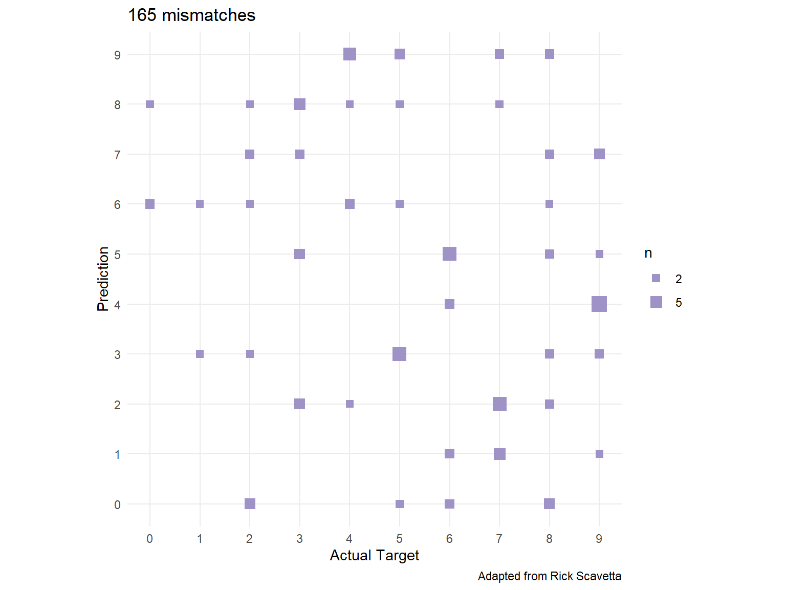

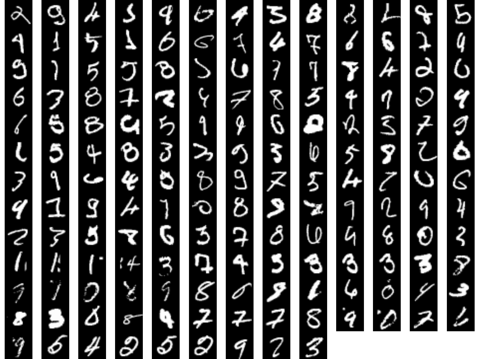
Visualize missed predictions

Lastly, lets check out those mispredicted digits.

missed <- which(predictions != actual)
plot_dim <- ceiling(sqrt(length(missed)))

par(mfrow = c(plot_dim, plot_dim), mar = c(0,0,0,0))
for (i in missed) {
  plot(as.raster(mnist$test$x[i,,], max = 255))
}

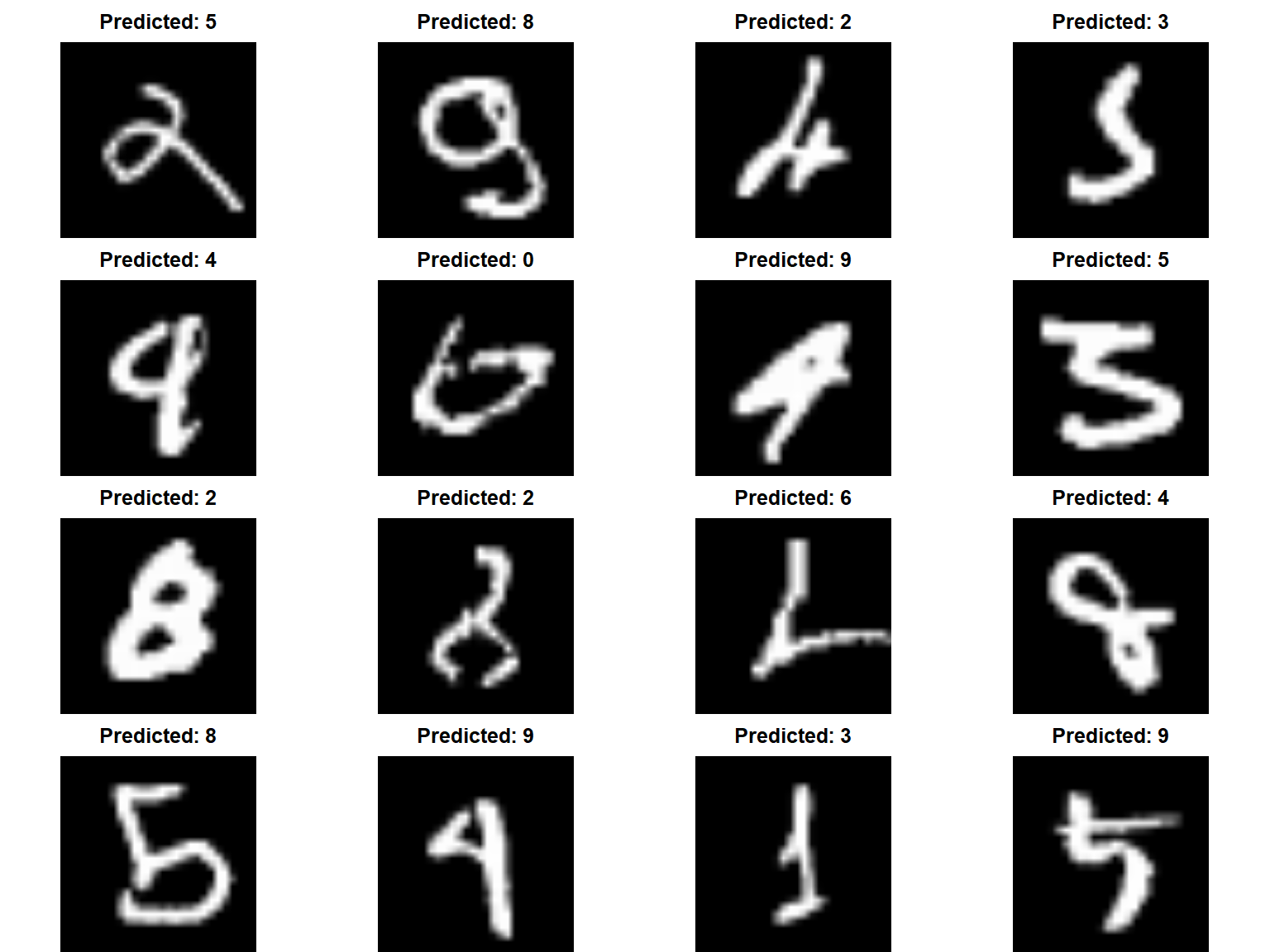
If we look at the predicted vs actual we can reason about why our model mispredicted some of the digits.

par(mfrow = c(4, 4), mar = c(0,0,2,0))

for (i in missed[1:16]) {
  plot(as.raster(mnist$test$x[i,,], max = 255)) 
  title(main = paste("Predicted:", predictions[i]))
}

Key takeaways

Follow these steps and guidelines when tuning your DL model:

1. Prepare data
   • data needs to be shaped into the right tensor dimensions
   • data should be scaled so they don’t trigger exploding gradients
2. Balance batch size with a default learning rate so that…
   • your learning curve is not too noisy
   • the training compute time is sufficient
3. Tune the adaptive learning rate optimizer
   • compare SGD+momentum with RMSprop & Adam
   • assess learning rates on log scale between [1e-1, 1e-7]
4. Add callbacks to control training
   • use early stopping for more efficient training
   • use an adaptive learning rate callback to have more control of the learning rate
5. Explore model capacity
   • compare adding width vs depth (consider loss vs. training time)
   • be smart with your experiments (use tensorboard callback!)
6. Regularize overfitting
   • weight decay controls magnitude of weights; start by assessing values btwn 0.1, 0.01, …, 0.0001
   • dropout minimizes happenstance patterns from noise; typical values range from 0.2-0.5.
7. Iterate, iterate, iterate!

References

Workshops

• Deep learning with R Summer course
• Deep learning with keras and Tensorflow in R (Rstudio conf. 2020)

Books

• Deep learning with R, 2nd edition. F. Chollet